We will learn about magnetic anomalies and how to contour them. We will interpret magnetic anomalies in terms of subsurface structure and rock magnetic properties.
Geoscientists collect magnetic data all over the world, mostly to learn more about the geology of the Earth's subsurface. In this module you will learn about magnetic anomalies and how to interpret them. The interpretation ranges from qualitative interpretation of contour maps of magnetic data to the use of numerical models to compare observed and calculated anomalies. One of the spectacular magnetic anomalies you will interpret is from Aso caldera, a giant Quaternary caldera on the island of Kyushu, Japan.
Aso caldera
Aso caldera erupted about 90 ka with such volume and force that pyroclastic density currents spread across the entire northern part of Kyushu, now home to more than 30 million people. The eruption left a giant ignimbrite deposit over much of the island and a tephra (volcanic ash) deposit that spread over all of Japan.
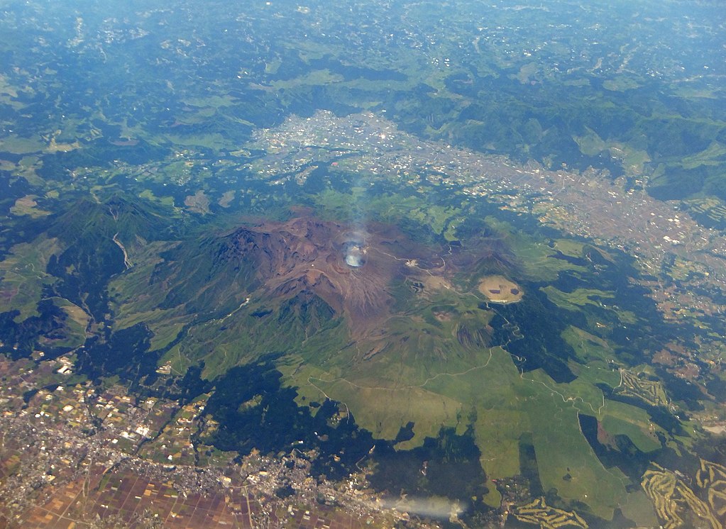
This is an oblique aerial view of Aso caldera. The steaming vent in the center is Naka-dake, a basaltic shield volcano that has grown in the center of the caldera since the caldera formed about 90 Ka. Naka-dake erupted in 2019, indicating how active the caldera system remains. Aeromagnetic data you will use in the later part of this module were collected by flying an airplane over the caldera recording the variation in the magnetic field, at an elevation about the same as the airplane elevation at which this photo was taken (photo from Wikipedia).
The eruption left a large hole in the ground - the Aso caldera. The caldera formed when so much magma erupted explosively that the roof over the magma chamber collapsed into the void left by the erupted magma. The caldera is about 20 km in diameter.
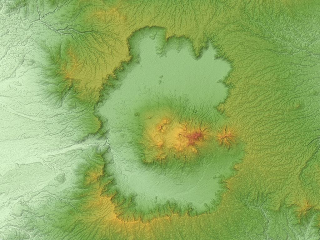
This shaded relief digital elevation model (taken from Wikipedia) gives an excellent perspective on the magnitude of collapse of the caldera during the 90 ka eruption. The high ground in the center of the caldera is the active Naka-dake. Many craters are visible in the topography of Naka-dake. Also note the river that flows to the west out of the caldera. During the 90 ka eruption, much pyroclastic material flowed in this direction. There is now a geologically active fault trending roughly parallel to the river which slipped in a M7 earthquake in 2016.
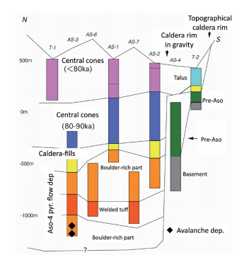
Big as the caldera is, it is actually mostly filled by the ignimbrite (pyroclastic rocks also called welded tuff) that erupted 90 Ka. The boreholes reveal avalanche deposits, welded tuff (ignimbrite) and caldera fill related to the eruption. No borehole has reached the base of this ignimbrite. Central cones like Naka-dake make a thick layer on top of the 90 ka intra-caldera fill.
Japanese scientists have drilled deep boreholes into Aso caldera and logged the change in lithostratigraphy within the caldera. The color bars represent lithostratigraphic logs of rock type as a function of depth in boreholes drilled into the caldera. Note that scientists identify welded ignimbrite (welded tuff) within the caldera at a depth of about 1200 m below the surface. It is possible that this welded ignimbrite layer is the cause of a giant magnetic anomaly associated with the caldera (Picture from a paper by S. Nakada, 1993).
Introduction to magnetic anomalies
Magnetic anomalies are variations in the Earth's magnetic field that occur because rocks, like basalts and andesites, contain magnetic minerals. The rocks become magnetized in the Earth's magnetic field and the strength of their magnetization (measured in units of ampere per meter) is proportional, roughly, to the percentage of magnetic minerals in the rock. Because magnetized rocks create magnetic anomalies, we can map magnetic anomalies and "see" into the Earth, even where the magnetized rocks are completely buried.
The strength of the Earth's magnetic field is measured in units of nanoTeslas (nT). The strength of the Earth's field varies with latitude (distance from the magnetic poles) from roughly 20,000 nT near the equator to roughly 60,000 nT near the poles. Locally, variation of 100s to 1000s of nanoTeslas occur near rocks that have high magnetization (high magnetic mineral content).
The variation in the Earth's magnetic field strength is measured with a magnetometer. Magnetometers can be carried across an area, flown by airplane, helicopter or drone, or towed behind a boat. When the magnetometer is carried by an aircraft the survey is called an aeromagnetic survey. Aeromagnetic surveys are particularly efficient for mapping magnetic anomalies over large areas. Magnetic surveys are also carried out by spacecraft to map the magnetic anomalies of the Moon and other planets.
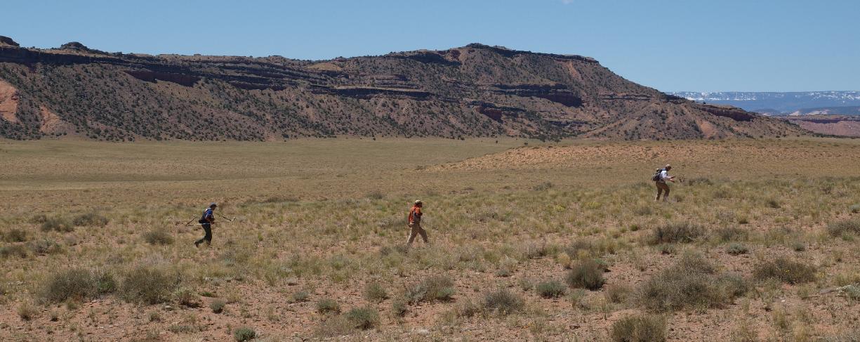
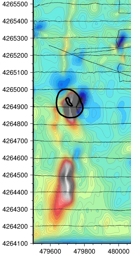
USF students making a magnetic map in the San Rafael Desert (UT). The student in front is using a GPS to keep the survey on an E-W line. The student in the back is carrying a magnetometer and GPS and is monitoring change in the magnetic field as he walks across the landscape. The rocks are red sandstones that have few magnetic minerals and hence low magnetization. Basaltic rocks intrude into the sandstone in this area, creating magnetic anomalies even if the basalt does not crop out at the surface.
The magnetic map of the area shown in the photo (above). The students in the photo are walking along an E-W line, at about 4265000 N. This magnetic map has very large amplitude magnetic anomalies (contour interval 100 nT) revealing the locations of basaltic dikes and sills buried beneath the surface within the sandstone. The black circles on the magnetic map corresponds to the slight topographic rise seen in the photo. Basalt crops out at this location and it is interpreted to be a volcanic conduit (neck) through which magma flowed upward toward the surface when the area was volcanically active. The dikes and sills trend N-S through this conduit area.
Modeling magnetic anomalies
Once a magnetic anomaly is mapped it is possible to interpret the map to guess about the subsurface features that cause the magnetic anomaly. This is a guess because different geometries and different magnetization can cause similar magnetic anomalies. Nevertheless, with additional geologic information it is often possible to interpret magnetic anomalies quite precisely.
Interpretation of magnetic anomalies starts with understanding the Earth's magnetic field is a vector. The vector of the Earth's magnetic field has a magnitude (nT) and a direction. The angle of the magnetic field with respect to the geographic North Pole is called the declination of the magnetic field (you use the declination to correct compass readings to True (geographic) North). Declination has units of degrees or radians. The angle of the magnetic field with respect to horizontal (approximately the Earth's surface) is called the magnetic inclination (units of degrees or radians), In the northern hemisphere, the inclination is positive, meaning the vector points into the Earth.
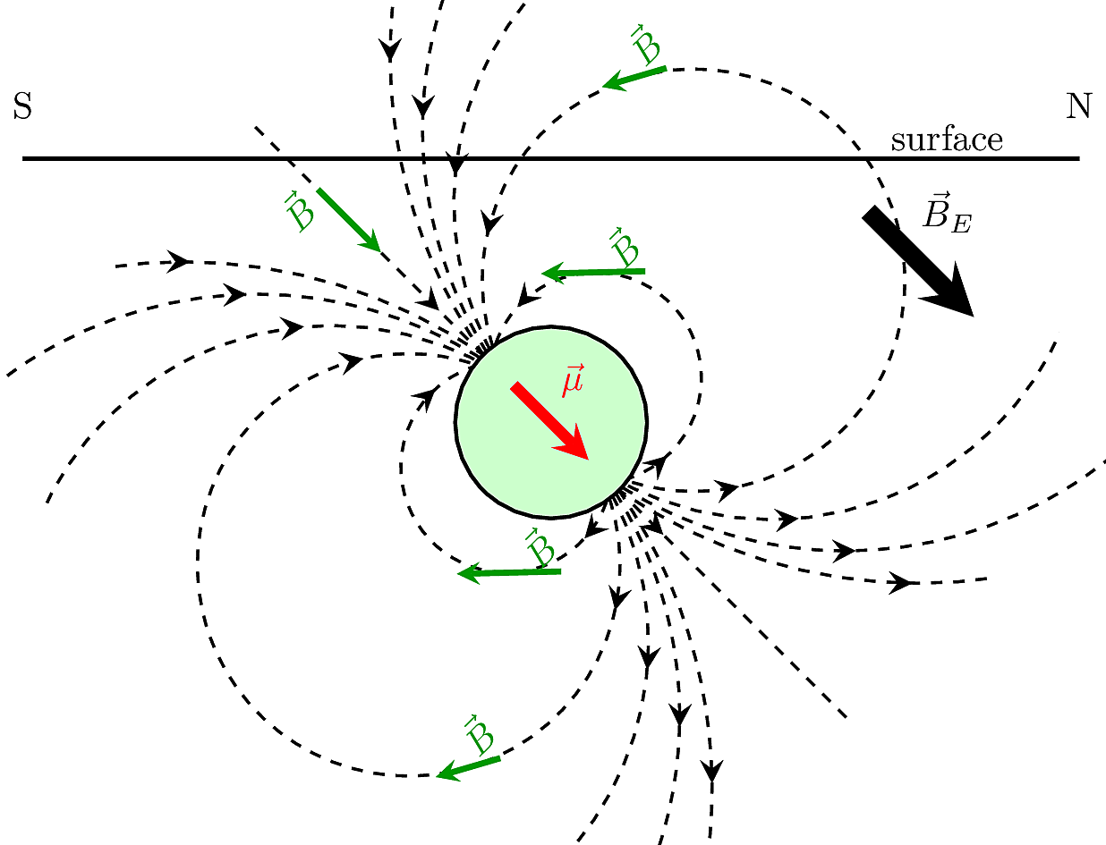
This figure shows the Earth's magnetic field, $\vec B_E$, with positive inclination (into the Earth). This vector is the normal Earth's magnetic field. The magnetic properties of the body (green sphere), cause it to become magnetized in the Earth's field, the vector $\vec \mu$. The size of $\vec \mu$ depends on the amount of magnetic material in the body and the strength of the external magnetic field. The magnetization is the length of the vector $\vec \mu$. The vector is called the magnetic dipole moment or the vector of magnetization.
Natural magnetic anomalies in the shallow Earth's crust are caused by the interaction of the Earth's magnetic field with rock bodies that contain magnetic minerals. The Earth's magnetic field (large black arrow, $\vec B_E$) is shown with positive inclination. The green circle represents a magnetized spherical rock body. The red arrow is the vector of magnetization ($\vec \mu$), also called the magnetic dipole moment. The vector of magnetization creates a magnetic field (dashed lines) around the sphere and a magnetic anomaly at the surface. The magnetic anomaly (green arrows) add to the Earth's magnetic field on the south side of the sphere, and subtract from the Earth's magnetic field on the north side of the sphere.
The vector of magnetization (magnetic dipole moment) creates a magnetic field around the magnetic body. The green arrows, $\vec B$, show the magnetic field created by the body. The change in orientation of this induced magnetic field is represented by lines of magnetic force (dashed lines with arrows). The density of the lines of magnetic force are proportional to the strength of the induced magnetic field. Note that the induced magnetic field (dashed lines) adds or subtracts from the Earth's field (big black arrow) depending on where the field is measured at the surface, relative to the position of the buried magnetized rock.
At the surface, lines of force converge and are oriented in or nearly in the direction of the Earth's field, $\vec B_E$, on the south side of the magnetized sphere. These induced lines of force add to the Earth's field, creating a positive magnetic anomaly. That is, magnetic measurements made at the surface on the south side of the sphere would be larger than one would expect if the sphere was not there.
Magnetic lines of force have the opposite or nearly opposite orientation on the surface north of the magnetized sphere. These induced lines of force subtract from the Earth's field, creating a negative anomaly on the north side of the sphere. The magnetized sphere creates a positive magnetic anomaly on its south side, and creates a negative anomaly on its north side.
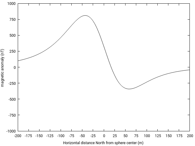
The lines of force are less dense on the north side of the sphere than on the south side. Given the inclination of the Earth's magnetic field, the lines of force converge at a shallower depth on the south side and so a stronger magnetic anomaly is created at the surface. The amplitude of the positive magnetic anomaly, measured at the surface and plotted on the graph, is larger than the amplitude of the negative anomaly on the north side of the magnetized sphere.
This is the magnetic anomaly that would be observed by making a magnetic survey along the profile N-S profile line over the magnetized (green) sphere.
Magnetic anomalies can be calculated for rock bodies of different shapes and for different inclinations, declinations, and magnetizations. The following canvas illustrates the calculation of a magnetic anomaly due to a buried prism, like a lava flow or igneous sill. The prism is assumed to extend in and out of the screen by 1000 m. Use the mouse to change the depth of the prism and use the slider bar to change the inclination of the magnetic field.
Notice that the shape of the magnetic anomaly changes with inclination and the amplitude of the magnetic anomaly changes with depth. The positive and negative magnetic anomaly maxima correspond to the edges of the prism at most inclinations. This is only strictly true for shallow, thin magnetic bodies, like this one.
Magnetic anomaly of Aso caldera
Ignimbrites have variable magnetization depending on their composition, temperature of emplacement and fabric. Welded facies of Aso ignimbrite have extremely high magnetization, reportedly 1-9 amp/m. It is not surprising then, that a large magnetic anomaly is located within the caldera, where pyroclastic material accumulated at sufficient rate and to sufficient depth to result in a thick welded section. In fact, the Aso magnetic anomaly is the largest amplitude magnetic anomaly on the island of Kyushu, with a peak-to-peak amplitude of approximately 1700 nT.
The main part of the aeromagnetic anomaly is located entirely within the caldera. The causative body is a plate-like source, consistent with the interpretation that the anomaly is caused by a layer of magnetized welded ignimbrite.
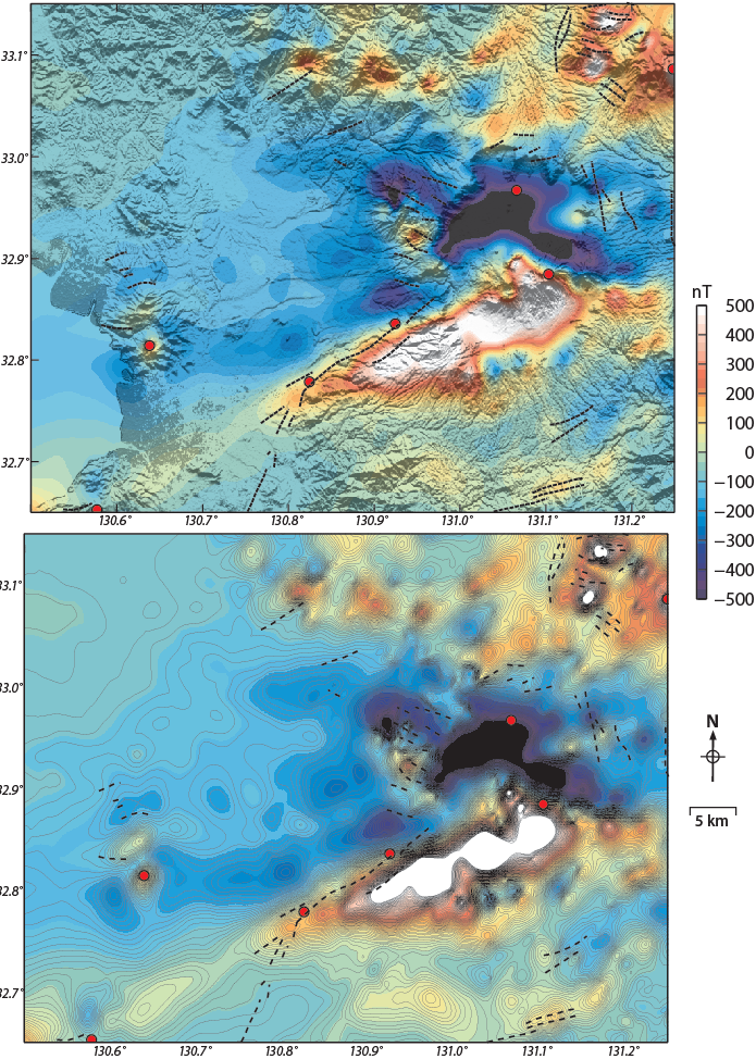
Regional aeromagnetic data for the area around Aso caldera, superimposed on a shaded-relief digital elevation model (top) and contoured (bottom). Aeromagnetic data are shown for a uniform flight elevation of 1500 m above the surface. A prominent dipolar (positive and negative) magnetic anomaly is centered within the caldera, west of Naka-dake (red dot near the center of the caldera where the magnetic anomaly changes from positive to negative). The magnetic anomaly extends southwest of the caldera, along the Futagawa fault zone segment, which experienced a M7 earthquake in 2016. Other vents in the volcano database of Japan are shown as red dots including Omine and Akai volcanoes, west of the caldera boundary. Faults, from the Quaternary fault database of Japan are shown as dashed lines, including the Futagawa fault zone segment, which connects Akai and Omine volcanoes and trends into Aso caldera. Figure courtesy of L. Connor.
The aeromagnetic anomaly gives insight into the nature of the ignimbrite that fills the caldera.
Do the following:
Make a word document that contains this work. You will need pencils, eraser, protractor, ruler and graph paper (color pencils optional).
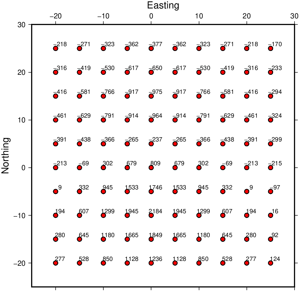
Magnetic maps can be difficult to interpret because a single body (buried prism!) creates both positive and negative anomalies. Because the positive and negative anomalies are associated with the same source, such magnetic anomalies are called dipolar. This is a map of magnetic readings that reveals a dipolar magnetic anomaly. The units on the map border are in meters. A magnetic body is buried in the map area. The body is a prism (square in map view) and extends from -10 to 10 East and from -10 to 10 N. The body is magnetized in the Earth's magnetic field with declination of $0^{\circ}$ and inclination of $45^{\circ}$. The top of the body is buried 10 m below the surface and the bottom is 30 m below the surface.
Here is the magnetic map to contour. The red circles show magnetic reading locations. The numbers are magnetic anomaly values in nanoTesla. You can right-click on the map to "view image" in a separate window, or right-click and "save as...". You can print the map from this window so you can contour it.
Contour the magnetic map. Be sure to choose an appropriate contour interval and use the same contour interval for the entire map. You can color-shade the map to make the magnetic anomaly stand out.
Draw the outline of the prism (square) on the map.
On graph paper, draw a N-S profile of the magnetic anomaly along easting line 0. Show the inclination of the Earth's magnetic field on your profile. Show the vertical edges of the prism on your profile.
What is the relationship between the dipolar (positive and negative) magnetic anomaly and the edges of the prism? Refer to both map and profile, as well as information on this web-page about the vector of magnetization, induced magnetic fields and lines of force.
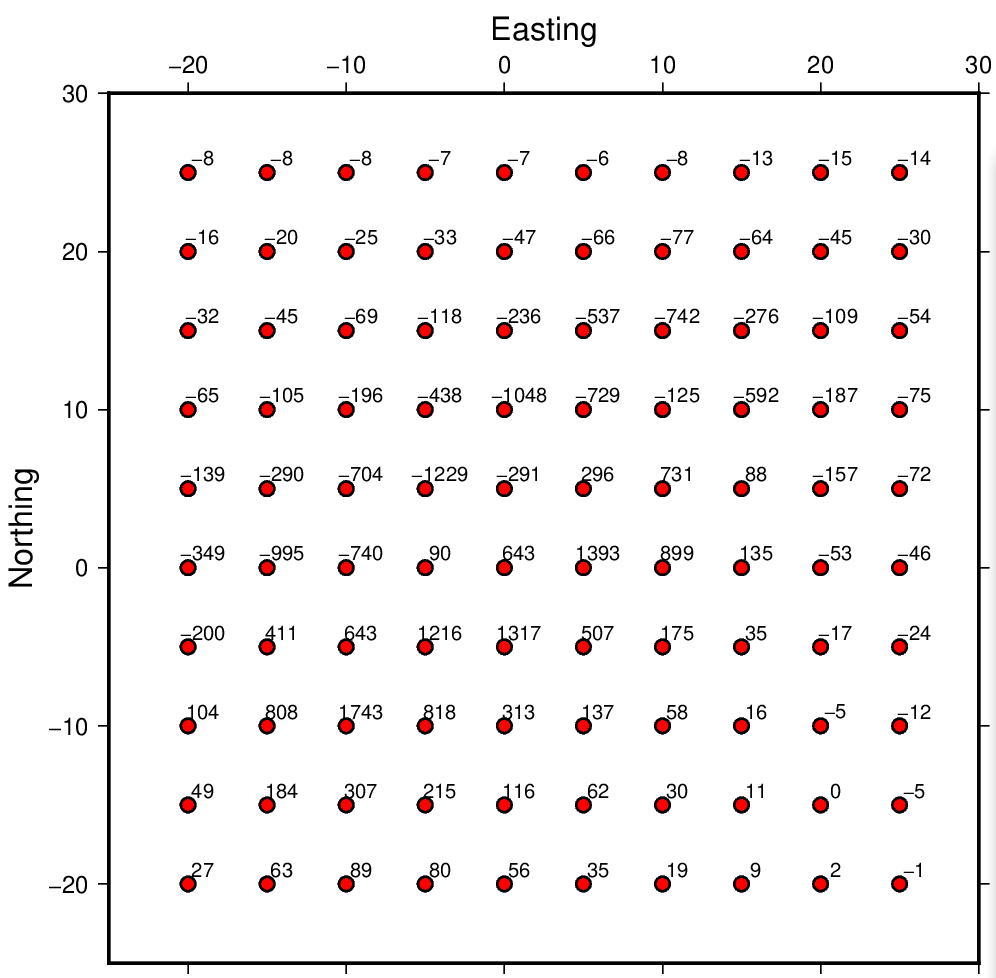
This is another map of magnetic readings from a different area.
Here is a second magnetic map to contour. The red circles show magnetic reading locations. The numbers are magnetic anomaly values in units of nanoTesla. You can right-click on the map to "view image" in a separate window, or right-click and "save as...". You can print the map from this window so you can contour it.
Contour the magnetic anomaly on this map. As before, be sure to choose an appropriate contour interval and use the same contour interval for the entire map. Color-shade the map to make the dipolar magnetic anomaly stands out.
On graph paper, draw a N-S profile of the magnetic anomaly along easting line 0.
Study the positive and negative anomalies on this map. Try to outline the body that causes the magnetic anomaly on your plot of contoured magnetic readings. Make sure you compare with your answer to question #1.
Develop a model for the aeromagnetic anomaly observed at Aso caldera. You will try to outline the lateral extent (in map view) of the magnetized intra-caldera fill within the caldera. You will model magnetic profile data to obtain a good qualitative fit between observed anomalies and the calculated magnetic anomaly.
Go to the Aso Caldera magnetic model and follow instructions to model the observed aeromagnetic anomaly.
Once you obtain a good fit save the model data to a file (use the save button!) AND save a copy of the map and one of the profiles by right-clicking and selecting "save image as...".
What is the depth, thickness and magnetization of the layer that causes the magnetic anomaly at Aso caldera? Does your model agree with the sparse borehole data about the depth and thickness of the intra-caldera welded ignimbrite? Explain your model and your estimates of the thickness and depth of the intra-caldera fill in a brief paragraph (three or four sentences).
Estimate the volume of the intracaldera welded ignimbrite using your polygon and thickness. You can estimate the area of the polygon first, using the perimeter of an irregular polygon. A simple formula for the area is:
$$A = \frac{1}{2} \sum_{k=0}^{n-1} (x_k y_{k+1} - y_k x_{k+1}) $$
Turn in your maps, models, and answers in a word document. Paste the images into the word document along with your Aso model output (question #3). Include answers to questions #1 and #2 by scanning the maps (if that is available to you) or by taking pictures of them. Make sure the picture or scan is clear enough to see your contour lines and include these figures in your word document.