Geologists estimate the volumes of deposits, often using sparse data. One way to compare the sizes of explosive volcanic eruptions is using the Volcano Explosivity Index (VEI), which depends mainly on the volume of tephra erupted. So to measure the "size" of an explosive eruption, it is necessary to estimate the volume of the tephra deposit. There are many techniques for estimating volume, but they all start with having map data!
Tephra
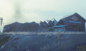
Tephra fallout occurs following explosive volcanic eruptions, when tephra particles (micron to decimeter in diameter) are carried aloft in volcanic plumes, advected by the wind, and sediment on to the surrounding countryside. The thickness (m) and loading (kg m$^{-2}$) of tephra fallout varies widely with distance from the source of the volcanic eruption and the intensity of the volcanic eruption. Following the most intense volcanic eruptions, tephra fallout may exceed 1 m thickness, or 1000 kg m$^{-2}$ in areas located within a few kilometers or tens of kilometers of the volcano. Tephra has densities ranging from approximately $800-1200$ kg m$^{-3}$, and so is much denser than snow. In addition, the load of tephra on roofs increases substantially when the tephra deposit saturates with rainwater. If not cleared off the roof, this load causes some buildings to collapse. Building collapse by tephra-loading has caused many fatalities during explosive volcanic eruptions.
Tephra fallout caused collapse of this poorly designed warehouse outside of Leon (Nicaragua) during the 1992 eruption of Cerro Negro volcano.
Isopach and isomass maps
Maps of geologic deposit thickness are usually called isopach maps (pronounced iso-pack). The contour lines on an isopach map connect areas of equal deposit thickness. Isopach maps are useful for determining deposit volume because one can sum the areas enclosed by different isopach contours to calculate total volume of the deposit.
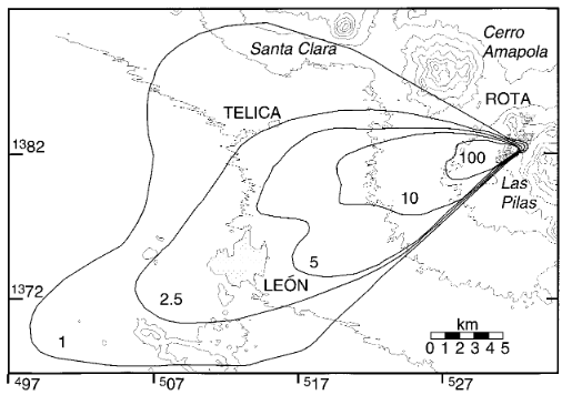
An isopach map of the tephra fallout deposit of the 1992 eruption of Cerro Negro volcano (Nicaragua). The thickness of the deposit is contoured in units of centimeters. The collapsed warehouse was located on the east side of the city of Leon, where tephra thickness was about 5 cm. Note that the contour interval is roughly logarithmic to account for the rapid change in deposit thickness with distance from the volcano.
Using this isopach map of Cerro Negro, one can find the area, $A_1$, enclosed by the 100 cm isopach, of estimated average thickness $T_1$. Then the volume represented by this isopach is:
$$V_1 = A_1 T_1 $$
The area enclosed by the 10 cm isopach is $A_2$ of average thickness $T_2$. Then the estimated deposit volume enclosed within this isopach is
$$V_1 + V_2 = A_1 T_1 + (A_2 - A_1) T_2 $$
Notice we do not want to account for the area $A_1$ twice, so this area is subtracted in the second term on the right-hand side of the equation. One can continue summing isopachs and their average thickness in this way until the deposit is too small to measure. Of course, it is often tricky to estimate the average thicknesses ($T_1, T_2$, etc.). Also, significant volume often extends beyond the last contoured isopach. So volcano scientists use a variety of methods to estimate deposit volume. These equations represent a useful approach to estimate minimum deposit volume.
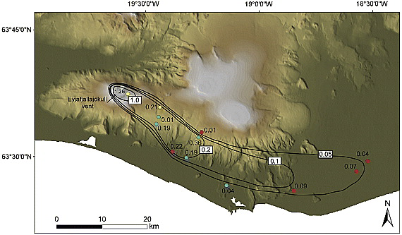
An isomass map is like an isopach map, but instead of contouring thickness of the deposit the mass load of the deposit is contoured, in units of mass per unit area. Using an isomass map of a tephra deposit, it is possible to estimate the total mass of the eruption, using the same method as outlined above for tephra volume estimated from contoured thickness measurements.
An isomass map of the tephra fallout deposit of the 2010 eruption of of Eyjafjallajokull volcano (Iceland). The mass loading of the deposit is contoured in units of kilogram per square meter. (Figure from Bonadonna et al. 2011, Journal of Geophysical Research).
June 1996 eruption of Ruapehu volcano, New Zealand
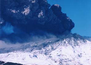
Ruapehu volcano erupted explosively in June 1996. Check out the Smithsonian web-page about Mt. Ruapehu for details about the volcano and accounts of the 1996 eruption.
Photo of the 1996 eruption of Mt. Ruapehu, one of the most frequently active volcanoes in New Zealand. Tephra is lofting into the atmosphere and being advected downwind forming a relatively narrow and thick deposit. (photo from Michigan Tech website)
The tephra emitted from the eruption was blown NE across the North Island of New Zealand. Bruce Houghton (University of Hawaii) and colleagues mapped the deposit all the way from Mt. Ruapehu to the north coast. In this exercise we will use their eruption data to estimate the volume of the deposit.
Much of the eruption deposit was quite thin. In these areas, the Houghton team gathered data by marking off a known area and sweeping up all the tephra in that area and weighing it, to report mass loading in mass per unit area. Assuming a deposit density of about 1000 kg m$^{-3}$ the mass loading can be converted to a deposit thickness:
$$ T = \frac{M}{A \rho} $$
where $T$ is the deposit thickness (m), $M$ is the mass (kg) in area $A$ and $\rho$ is the density of the deposit.
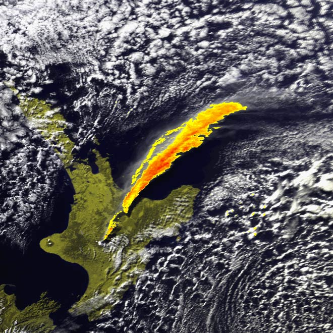
False color satellite image of the volcanic plume produced by the June 1996 eruption. The plume (orange colors) creates a reflective surface in some parts of the spectrum, which allows tracking the plume by satellite in some circumstances. The image shows how the volcanic plume trends across New Zealand's North Island and out to sea. (image from Wikipedia).
Do the following:
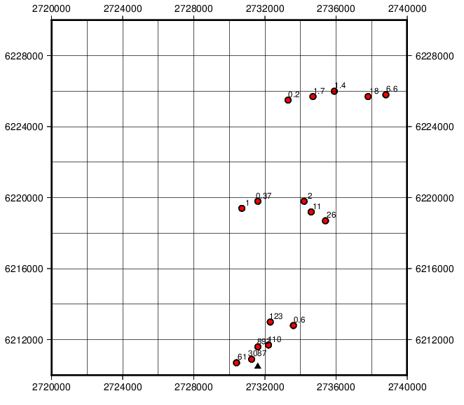
These map data show the mass loading (kilograms per square meter) of tephra deposited from the 1996 eruption relatively close to the volcano (called the proximal area of the deposit). The data are somewhat simplified from all the data collected at the time by Bruce Houghton and colleagues.
The red dots show sample locations for the tephra deposit and the numbers are in units of mass loading (kg m$^{-2}$). The location of the Ruapehu volcanic vent is indicated by the solid black triangle. The coordinates of the map are shown in the New Zealand topographic grid system (much like UTM) and are in units of meters.
Download and print the map. You can right-click on the image, save the map and print.
Note the range of mass loading values. Select a contour interval that is appropriate for these data. Consider using a logarithmic contour interval.
Contour the mass loading data. Note that the samples are relatively sparse, but you can also use the satellite image to infer that the deposit formed by deposition of tephra from a narrow volcanic plume blowing to the NE. Geologists are often faced with contouring relatively sparse data using assumptions about the deposit. Use dashed lines to indicate areas where you are particularly unsure of the position of the contours because the data are sparse.
The major axis of tephra dispersion is a line that can be drawn from the volcano through the thickest part of the deposit with increasing distance from the volcano. The thickness of the deposit decreases along the major axis of dispersion with increasing distance from the volcano, and also deposit thickness decreases orthogonal to the major axis of dispersion. Draw the major axis of dispersion on your contour plot. How thick is the deposit on the major axis of dispersion two kilometers from the volcanic vent and ten kilometers from the volcanic vent?
The following map shows the thickness of the tephra deposit (mm) over a much larger area (also mapped by Bruce Houghton and colleagues). The light gray map grid outlines areas that are 20 x 20 km. The ticks at the edge of the map are in 50 km intervals. Estimate the volume of the 1996 tephra deposit using this map.
Note that the box with big red circles and small yellow circles outlines an area on the map in square pixels. You can move the corners of the box by dragging the red circles with your mouse. This changes the area of the box. You can click on the yellow circles to add corners to the polygon to outline areas that are not rectangular. Find the scale of this map in units of pixels per square kilometer.
Drag the polygon corners and add corners to outline the approximate area (square pixels) within which the deposit is >100 mm, 10-100mm,...,0.01 -0.1 mm. You will likely need to reload the web-page from time to time to reset the polygon to its default position. Convert these areas from square pixels to square kilometers. Make a table of these values. You can use a spreadsheet (like Excel) to help make this table and perform subsequent calculations. Save an example of the isopach area for the 0.1 mm isopach. Right-click on the map after drawing this polygon to save the image.
Find an average thickness for each area you outlined. Because the thickness values are changing by orders of magnitude, it is best to use the average of the logarithms of the thickness range:
$$\log_{10} T_{avg} = \frac{\log_{10} (T_{max}) + \log_{10} (T_{min})}{2} $$
where $T_{avg}$ is the average thickness of the deposit inside the area of your polygon, $T_{min}$ and $T_{max}$ give the range of thicknesses. For >100 mm use an average thickness of 316 mm. That is, assume $T_{min} = 100$ mm and $T_{max}= 1000$ mm.
Calculate the volume represented by each polygon and sum these volumes to get the total volume of the deposit within the map area. Use Excel (or python for the adventerous) and document your calculation. Be careful though, you want to start with the volume of the polygon > 100 mm, then add only the additional area of the 10-100 mm polygon and so on (Hint: do not count the area of the >100 mm polygon twice!). Report your volume in cubic meters. What sources of error are associated with your volume estimate?
Turn in your answers to the questions using a word document. Scan your contoured isomass map and paste into your word document. Or, take a picture of the isomass map and insert in your word document. Include your Excel spreadsheet or python script. Be sure to show your work.