The Bouguer Slab
The Bouguer slab and Bouguer gravity correction explained
Introduction
What is the gravity anomaly due to an infinite horizontal slab, a horizontal unit of such great lateral extent, that it can be considered to be infinite?
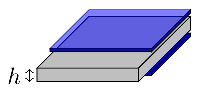
For an infinte horizontal slab (gray) of thickness $h$, the equipotential surface (blue) is uniform. Gravity on the equipotential surface, above and below the infinite slab, is uniform. Remarkably, the gravity anomaly due to the slab does not change with the distance of the equipotential surface from the slab, as explained by the math in the following.

Mathematical model
From Gauss's Law, \begin{align} \oint_S \vec g \cdot \vec n dA & = -4 \pi GM\\ M_S & = S \Delta \rho h\\ -2 S g & = -4 \pi G M_S\\ g & = 2 \pi G \Delta \rho h \end{align} where,
- $S$ is the unit surface area of the slab,
- $M_S$ is the mass of the slab per unit surface area
- $G$ is the gravitational constant
- $\Delta \rho$ is the density contrast between the slab and surrounding medium (surrounding rock)
- $h$ is the thickness of the slab
The Gaussian surface enclosing the slab is two times the surface area. One part of the hypothetical Gaussian surface is shown as the blue plate above the slab, the other part is the blue plate below the slab. Because the slab is infinite, the edges of the enclosing surface are not considered; only the surface above and below the slab need be considered.
The gravity anomaly due to the infinite horizontal slab does not depend on the distance, $r$, from the slab. We can think of this in terms of the divergence of the gravity field, which can be calculated in terms of $r$, \begin{align} \nabla \cdot \vec g & = \frac{\partial \vec g}{\partial r} \mathbf{ \hat r}\\ \nabla \cdot \vec g & = \frac{\partial }{\partial r} (2 \pi G \Delta \rho h) \mathbf{ \hat r}\\ \nabla \cdot \vec g & = 0 \end{align}
Physically, this means that the flux of gravity through the surface does not change with distance. So the gravity anomaly due to the infinite slab is the same 10 m from the slab as it is 1000 m away.
The formula for the infinite slab is used to calculate the simple Bouguer gravity correction (also known as Bullard A), where $h$ is replaced by the elevation difference between gravity stations.
TikZ code for the Bouguer slab figure
The LaTeX code (using TikZ) for drawing the picture of the Bouguer slab and its equipotential surface is given below.
\documentclass{article}
\usepackage{tikz}
\usepackage{tikz-3dplot}
\usetikzlibrary{calc,fadings,decorations.pathreplacing}
\usepackage{verbatim}
\usepackage{verbatim}
\usepackage[active,tightpage]{preview}
\PreviewEnvironment{tikzpicture}
\setlength\PreviewBorder{5pt}%

\begin{document}
\begin{tikzpicture}[scale=0.5]

% draw a condensor plate
\draw[fill=blue] (-1.5,-0.5,-2.5)--(-1.5,-0.5,0.5)--(1.5,-0.5,0.5)--(1.5,-0.5,-2.5)--cycle;
\draw[fill=blue] (1.5,-0.5,-2.5)--(1.5,-0.6,-2.5)--(1.5,-0.6,0.5)--(1.5,-0.5,0.5)--cycle;
\draw[fill=blue] (1.5,-0.6,0.5)--(-1.5,-0.6,0.5)--(-1.5,-0.5,0.5)--(1.5,-0.5,0.5)--cycle;

% draw a condensor plate
\draw[fill=lightgray] (-1.5,0,-2.5)--(-1.5,0,1.5)--(1.5,0,1.5)--(1.5,0,-2.5)--cycle;
\draw[fill=lightgray] (1.5,0,-2.5)--(1.5,-0.4,-2.5)--(1.5,-0.4,1.5)--(1.5,0,1.5)--cycle;
\draw[fill=lightgray] (1.5,-0.4,1.5)--(-1.5,-0.4,1.5)--(-1.5,0,1.5)--(1.5,0,1.5)--cycle;

% draw a condensor plate
\draw[fill=blue, opacity=0.5] (-1.5,0.2,-2.5)--(-1.5,0.2,0.5)--(1.5,0.2,0.5)--(1.5,0.2,-2.5)--cycle;
\draw[fill=blue] (1.5,0.2,-2.5)--(1.5,0.1,-2.5)--(1.5,0.1,0.5)--(1.5,0.2,0.5)--cycle;
\draw[fill=blue] (1.5,0.1,0.5)--(-1.5,0.1,0.5)--(-1.5,0.2,0.5)--(1.5,0.2,0.5)--cycle;
\draw [<->]  (-2.3,-.6,0)--node[left]{$h$} (-2.3,-1,0);

\end{tikzpicture}
\end{document}