gbox and the Buried Prism
Calculate the gravity anomaly due to a vertical-sided prism using the gbox algorithm
Contents
Introduction
gbox will calculate the gravity anomaly due to a vertical-sided prism with horizontal top and bottom and uniform density contrast. The gbox algorithm can be used to model gravity anomalies from geologic features that can be represented by prisms, such as sedimentary basins. More complex models can be built using multiple prisms.
Mathematical model

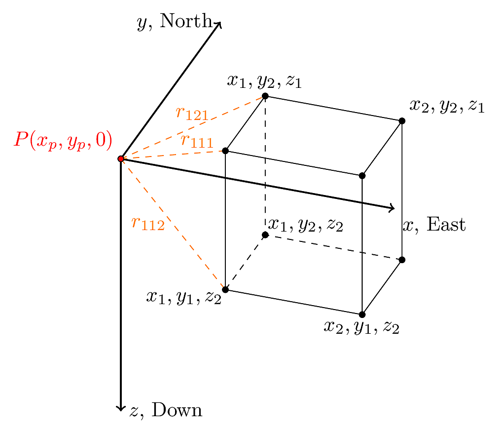
Based on the model above, gravity is observed at a point $P(x_p, y_p,z_p)$, where $x_p$ is the easting coordinate of the observation point, $y_p$ is the northing coordinate of the observation point, and $z_p = 0$ in this example is the elevation of the observation point. Coordinates of the gravity station are assumed to be in meters.
The edges of the prism, buried in the subsurface, are defined by the coordinates: $x_1$ - west side, $x_2$ - east side, $y_1$ - south side, $y_2$ - north side, $z_1$ depth to top of the prism, and $z_2$ - depth to bottom of the prism. Prism coordinates are also assumed to be in meters.
The following equations for calculating the gravity anomaly due to a vertical sided prism are from Blakely(1996).
If $P(0,0,0)$, then the gravity anomaly due to the prism is $$\Delta g = \Delta \rho G \int_{x_1}^{x_2} \int_{y_1}^{y_2} \int_{z_1}^{z_2} \frac{z}{(x^2+y^2+z^2)^{3/2}} dx dy dz$$
Plouff(1976) showed that this integral is approximately $$\Delta g = \Delta \rho G \sum_{i=1}^{2} \sum_{j=1}^{2} \sum_{k=1}^{2} \mu_{ijk} \left[ z_k \tan^{-1} \left ( \frac{x_i y_j} {z_k R_{ijk}} \right ) - x_i \ln(R_{ijk} + y_j) - y_j \ln(R_{ijk} + x_i) \right ] $$ where, \begin{align} R_{ijk} & = \sqrt{x_i^2 + y_j^2 + z_k^2}\\ \mu_{ijk} & = (-1)^i (-1)^j (-1)^k \end{align} $\Delta \rho$ is the density contrast and $G$ is the gravitational constant.
In practice, the relative position of the prism with respect to the observation point is determined, $$\Delta x_1 = x_p - x_1$$ $$\Delta x_2 = x_p - x_2$$ $$\Delta y_1 = y_p - y_1$$ $$\Delta y_2 = y_p - y_2$$ $$\Delta z_1 = z_p - z_1$$ $$\Delta z_2 = z_p - z_1$$ Distances are defined from the observation point to the corners of the prism. For example, $$r_{111} = \sqrt{\Delta x_1^2 + \Delta y_1^2 + \Delta z_1^2}$$ $$r_{121} = \sqrt{\Delta x_1^2 + \Delta y_2^2 + \Delta z_1^2}$$ $$r_{112} = \sqrt{\Delta x_1^2 + \Delta y_1^2 + \Delta z_2^2}$$ or more generally, $$r_{ijk} = \sqrt{\Delta x_i^2 + \Delta y_j^2 + \Delta z_k^2}$$
We make the following calculations for each corner $\Delta x_i$, $\Delta y_j$, and $\Delta z_k$, \begin{align} \\ a & = \tan^{-1} \frac{\Delta x_i \Delta y_j}{\Delta z_k r_{ijk}}\\ \\ b & = \ln \left( r_{ijk} + \Delta y_j \right) \\ c & = \ln \left( r_{ijk} + \Delta x_i \right) \end{align} If the value of $a$ is less than zero, then add $2 \pi$.
- If $a < 0$, $a = a + 2 \pi$.
A variable, $s$ is introduced to alter the sign of the distance, $d_{ijk}$ in the following formula depending on the values of the indices $i$, $j$, and $k$ (refer to the above figure).
- If $i = 1, s_i = -1$
- If $i = 2, s_i = 1$
- If $j = 1, s_j = -1$
- If $j = 2, s_j = 1$
- If $k = 1, s_k = -1$
- If $k = 2, s_k = 1$
- $\Delta g$ is the gravity anomaly (meters per second squared)
- $\Delta \rho$ is the density contrast (kg per cubic meter)
- $G$ is the gravitational constant, $6.67 \times 10^{-11} \textrm{ m}^3 \textrm{ kg}^{-1} \textrm{ s}^{-2}$
Model assumptions
The gbox model assumes:
- The observation point is located outside the prism.
- The edges of the prism are parallel to the $x$, $y$ and $z$ axes, respectively.
- The prism is characterized by a single density contrast.
Calculate the gravity using C
Below is a C function that calculates the gravity anomaly at one point due to one prism.
#include < math.h >
#include < stdio.h >

#define gamma 6.670e-11L
#define twopi 6.2831853L
#define si2mg 1.0e5L
#define G_TEMP ((gamma) * (si2mg) )
#define SMALL 1e-10L

  /**********************************************************************
    Function gbox computes the vertical attraction of a
    rectangular prism.  Sides of prism are parallel to x,y,z axes,
    and z axis is vertical down.

    Input parameters:
    Observation point is (x0,y0,z0).  The prism extends from x1 (west)
    to x2(east), from y1(south) to y2(north), and from z1(depth to top)
    to z2(depth to bottom)
    in the x, y, and z directions, respectively.

    Distance units in meters.

    x is positive east
    y is positive north
    z is positive down

    Density of prism is rho. Thuis is the density contrast between
    the prism and surrounding rock.  rho in units of kg/(m**3).

    Output parameters:
    Vertical attraction of gravity, g, in mGal.

    Modified from Blakely, 1997, subroutine B.6
    Translated to C by L. Connor

  **********************************************************************/
double gbox(double *x0,double *y0,double *z0,double *x1,double *y1,double *z1,double *x2,double *y2,double *z2,double *rho) {

  int x,y,z;
  double sum;
  double  rijk, ijk;
  double arg1, arg2, arg3;
  double  xs[2],ys[2],zs[2],isign[2];
  double g;

  xs[0] = *x0 - *x1;
  ys[0] = *y0 - *y1;
  zs[0] = *z0 - *z1;
  xs[1] = *x0 - *x2;
  ys[1] = *y0 - *y2;
  zs[1] = *z0 - *z2;
  isign[0] = -1.0;
  isign[1] = 1.0;

  sum = 0.0;
  for (x = 0; x < 2; x++) {
    for (y = 0; y < 2; y++) {
      for (z = 0; z < 2; z++) {
        rijk = sqrt(xs[x]*xs[x] + ys[y]*ys[y] + zs[z]*zs[z]);
        ijk = isign[x]*isign[y]*isign[z];
        arg1 = atan2((xs[x]*ys[y]),(zs[z]*rijk));
        if (arg1 < 0.0) arg1 = arg1 + twopi;
        arg2 = rijk+ys[y];
        arg3 = rijk+xs[x];
        if (arg2 <= 0.0) arg2 = SMALL;
        if (arg3 <= 0.0) arg3 = SMALL;
        arg2 = log(arg2);
        arg3 = log(arg3);
        sum += ijk*(zs[z]*arg1-xs[x]*arg2-ys[y]*arg3);
      }
    }
  }
  g = *rho * sum * G_TEMP;
  return g;
}
Some additional code is needed to execute the above C function. A main C driver routine, run.c, will:
- initialize the location of the prism,
- set the density contrast between the prism and the surround,
- set up a location grid where the gravity will be calculated,
- call the gbox function to calculate the gravity at each grid location
- output the value of gravity calculated
In this example,
run.c provides a calculation involving points transecting the center of a single prism.
#include < math.h >
#include < stdio.h >

/****************************************
run.c provides an example calculation
involving points transecting the center
of a single prism.

COMPILE:
  gcc -o run run.c gbox.c -lm

USAGE:
  ./run > outfile.dat
*****************************************/

double gbox(double *x0,double *y0,
            double *z0,double *x1,
            double *y1,double *z1,
            double *x2,double *y2,
            double *z2,double *rho);

int main() {
  double grav, x, y, z, x1, x2, y1,y2,z1,z2, rho;

  x2= 573000.0; /*east side of box*/
  x1= 572000.0; /*west side of box */
  y2= 3756000.0; /*north side of box */
  y1= 3755000.0; /* south side of box */
  z1= 100.0; /*depth to top */
  z2= 500.0; /*depth to bottom */
  rho = -300.0; /*density contrast */
  y= 3755500.0;
  z = 0.0;

  for (x = 570000; x < 575000; x+=100) {
    grav = gbox(&x, &y, &z, &x1, &y1, &z1, &x2, &y2, &z2, &rho);
    fprintf (stdout, "%lf %lf\n", x, grav);
  }
return (0);
}
C is a compiled language and the source code must be compiled into a single executable file before it can be used. The C compiler, gcc on a Linux computer, can be used to compile the code into an executable that can be run from the command line. To compile type:
gcc -Wall run.c gbox.c -lm -o run
./run > outfile.dat
The output file outfile.dat is listed below:
570000.000000 -0.015767
570100.000000 -0.017856
570200.000000 -0.020330
570300.000000 -0.023285
570400.000000 -0.026841
570500.000000 -0.031162
570600.000000 -0.036461
570700.000000 -0.043034
570800.000000 -0.051283
570900.000000 -0.061775
571000.000000 -0.075319
571100.000000 -0.093093
571200.000000 -0.116847
571300.000000 -0.149248
571400.000000 -0.194445
571500.000000 -0.259058
571600.000000 -0.353879
571700.000000 -0.496837
571800.000000 -0.717973
571900.000000 -1.065102
572000.000000 -1.572005
572100.000000 -2.074281
572200.000000 -2.406937
572300.000000 -2.601842
572400.000000 -2.703135
572500.000000 -2.734492
572600.000000 -2.703135
572700.000000 -2.601842
572800.000000 -2.406937
572900.000000 -2.074281
573000.000000 -1.572005
573100.000000 -1.065102
573200.000000 -0.717973
573300.000000 -0.496837
573400.000000 -0.353879
573500.000000 -0.259058
573600.000000 -0.194445
573700.000000 -0.149248
573800.000000 -0.116847
573900.000000 -0.093093
574000.000000 -0.075319
574100.000000 -0.061775
574200.000000 -0.051283
574300.000000 -0.043034
574400.000000 -0.036461
574500.000000 -0.031162
574600.000000 -0.026841
574700.000000 -0.023285
574800.000000 -0.020330
574900.000000 -0.017856
Plotting the output using gnuplot
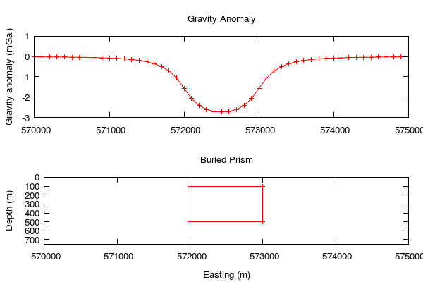
Use gnuplot to plot the profile and the cross section of the prism.
############################
# USAGE:
# type on the command line
# gnuplot gbox.gnu
############################

set terminal pngcairo  enhanced font "arial,10" fontscale 1.0 size 600, 400
set output 'gbox_profile.png'
set multiplot layout 2,1

# Axes label
set ylabel 'Gravity anomaly (mGal)'

# Axes ranges
set xrange [570000:575000]
set yrange [-3:1]

# Axes tics
set xtics 1000
set ytics 1

set title 'Gravity Anomaly'
plot  "outfile.dat" using 1:2 with linespoints lt rgb "red" notitle
set xlabel 'Easting (m)'
set ylabel 'Depth (m)'
set yrange [750:0]
set ytics 100
set title 'Buried Prism'
plot  "vertex.dat" using 1:2 with linespoints lt rgb "red" notitle
unset multiplot
The file vertex.dat contains the vertices of the buried prism, the corners (coordinates) of the prism in cross section:
572000 100
573000 100
573000 500
572000 500
572000 100
(bottom plot).

Drawing with LaTeX and TikZ
The following LaTeX and TikZ code draws the figure of the model geometry presented at the top of the page.
\documentclass[tikz, border = 1mm]{standalone}

\usepackage{tikz-3dplot}
\usetikzlibrary{shapes}

\begin{document}
\tdplotsetmaincoords{60}{110}

\begin{tikzpicture}[scale=5,tdplot_main_coords]
\coordinate (P) at (0,0,0);
\coordinate (A) at (-0.9, 0.2, -0.2);
\coordinate (B) at (-0.5, 0.2, -0.2);
\coordinate (C) at (-0.5, 0.7, -0.2);
\coordinate (D) at (-0.9, 0.7, -0.2);

\coordinate (Ap) at (-0.9, 0.2, -0.75);
\coordinate (Bp) at (-0.5, 0.2, -0.75);
\coordinate (Cp) at (-0.5, 0.7, -0.75);
\coordinate (Dp) at (-0.9, 0.7, -0.75);

\draw[thick,->] (0,0,0) -- (-1,0,0) node[anchor=east]{$y$, North};
\draw[thick,->] (0,0,0) -- (0,1,0) node[anchor=north west]{$x$, East};
\draw[thick,->] (0,0,0) -- (0,0,-1) node[anchor=west]{$z$, Down};
\draw[] (A)--(B);
\draw[] (B)--(C);
\draw[] (C)--(D);
\draw[] (D)--(A);
\draw[dashed] (Ap)--(Bp);
\draw[] (Bp)--(Cp);
\draw[] (Cp)--(Dp);
\draw[dashed] (Dp)--(Ap);
\draw [] (D) -- (Dp);
\draw [] (C) -- (Cp);
\draw [dashed] (A) -- (Ap);
\draw[] (B) -- (Bp);
\draw[dashed, orange] (P) -- node[above]{$r_{121}$}(A);
\draw[dashed, orange] (P) -- node[above right]{$r_{111}$}(B);
\draw[dashed, orange] (P) -- node[left]{$r_{112}$}(Bp);

\node[anchor=south] at (A) {$x_1, y_2, z_1$};
\node[anchor=north east, inner sep = 1pt] at (Bp) {$x_1, y_1, z_2$};
\node[anchor=south west, inner sep = 1pt] at (Ap) {$x_1, y_2, z_2$};
\node[anchor=south west] at (D) {$x_2, y_2, z_1$};
\node[anchor=north] at (Cp) {$x_2, y_1, z_2$};

\draw[fill=black, tdplot_screen_coords] (A) circle [radius=0.01];
\draw[fill=black, tdplot_screen_coords] (B) circle [radius=0.01];
\draw[fill=black, tdplot_screen_coords] (Bp) circle [radius=0.01];
\draw[fill=black, tdplot_screen_coords] (Ap) circle [radius=0.01];
\draw[fill=black, tdplot_screen_coords] (C) circle [radius=0.01];
\draw[fill=black, tdplot_screen_coords] (Cp) circle [radius=0.01];
\draw[fill=black, tdplot_screen_coords] (D) circle [radius=0.01];
\draw[fill=black, tdplot_screen_coords] (Dp) circle [radius=0.01];
\draw[fill=red, tdplot_screen_coords] (P) circle [radius=0.01];
\node[red, anchor=south east] (P) {$P(x_p, y_p, 0$)};

\end{tikzpicture}
\end{document}
Some References
- Blakely, R. J., 1996, Potential Theory in Gravity and Magnetic Applications, Cambridge University Press
- Plouff, D., 1976, Gravity and magnetic fields of polygonal prisms and application to magnetic terrain corrections. Geophysics 41: 727-741.
Citation
Connor, C. B. and L. J. Connor (2020) C-code for calculating the gravity anomaly due to a vertical-sided prism.Reference: https://gscommunitycodes.usf.edu/geoscicommunitycodes/public/geophysics/Gravity/gbox.php