Gravity Anomaly Due to a Thin Finite Horizontal Plate
Calculate the gravity anomaly due to a thin horizontal plate that has finite horizontal extent
Contents
Introduction
The gravity anomaly due to a horizontal plate of finite length, can be calculated based on an analytical solution of the gravitational potential. The model assumes the plate is thin and the gravitational attraction of the plate can be estimated by integrating along its length. That is, the gravitational attraction of a small mass on the top side of the plate is not different from the gravitational attraction of a small mass on the bottom side of the plate. Code is provided to perform this calculation.
A horizontal plate can be a good surrogate for the gravity anomaly associated with a sill or other horizontal geologic unit, with density contrast with the surrounding rock. In the geophysics literature horizontal finite plates are also call semi-infinite slabs. In a geophysics context these terms are the same.

Mathematical model
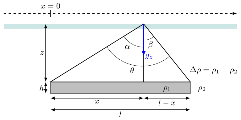
The formula for the gravity anomaly due to a horizontal plate of finite extent in the $x$ direction is: $$g_z = 2 G \Delta \rho h \left (\pi + \tan^{-1} \left [\frac{x}{z}\right ] + \tan^{-1}\left [\frac{l-x}{z}\right ] \right )$$ where:
- $z$ is the depth to the top of the horizontal plate,
- $x$ is the horizontal offset from the edge of the plate,
- $l$ is the length of the horizontal plate,
- $\Delta \rho$ is the density contrast between the plate and surrounding rock,
- $G$ is the gravitational constant.
Note, the horizontal plate is assumed to extend infinitely in the $y$ direction (in and out of the $x-z$ plane). Also, in this formulation, the background value of gravity is not zero, but is calculated as, $$ g_z = 2 G \Delta \rho h \pi$$ This makes it easier to understand the relationship between the formula for a finite horizontal plate and the Bouguer (infinite) slab, which is a horizontal plate that extends to infinity in E-W and N-S directions.
The infinite horizontal plate
The expression for the gravity anomaly from a horizontal plate going to infinity in one x-direction, is $$g_z = 2 G \Delta \rho h \left (\frac{\pi}{2} + \tan^{-1}\left [\frac{x}{z}\right ] \right )$$ this simple shape is sometimes referred to as a semi-infinite plate (or semi-infinite slab). The gravity due to an infinite plate (also called an infinite Bouguer slab) can be expressed as, $$g_z = 2 \pi G \Delta \rho h$$.
Model assumptions
This model assumes that:
- The plate extends infinitely in the strike direction (orthogonal to the x-z plane).
- The plate is thin; this thin plate is a good approximation to the prism if the thickness of the plate is less than the depth to the top of the plate.
- The plate is uniform and the density contrast between the plate and the surrounding rock (medium) is constant.
Calculate the gravity using perl
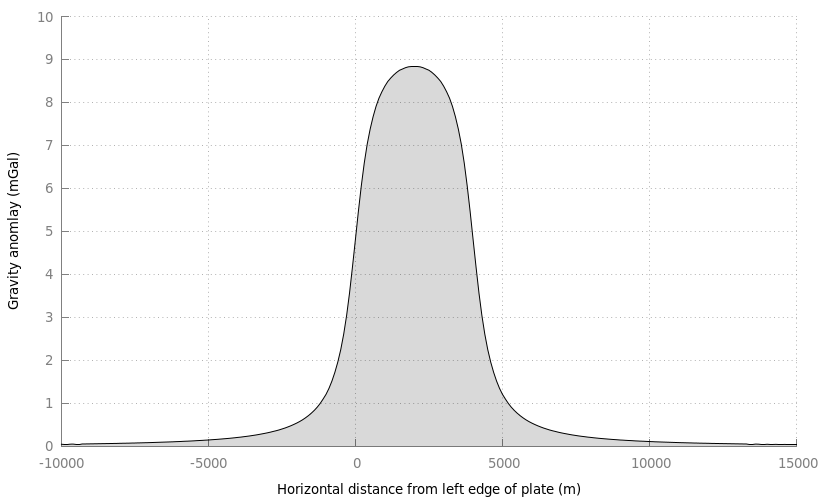
The following perl code demonstrates the calculation of the gravity anomaly due to a finite plate. Note that the expression $$g_z = 2 G \Delta \rho h \pi$$ is subtracted from the formula to plot the deviation of gravity from zero. This perl code creates the input file for the following plotting script. The perl script requires additional libraries that can be installed using the perl program cpan:
- Math::SigFigs
- Math::Trig
#!/usr/bin/perl

# command line USAGE: perl finite_plate.pl > finite_plate.dat

use warnings;
use strict;
use Math::SigFigs;
use Math::Trig;

######Main Code########
my $plate_length = 4000; #m
my $plate_depth = 500; #m
my $plate_thickness = 50; #m
my $plate_density_contrast = 500; #kg/m3
my $offset = 0.0;
my $gravity = 0.0;

for (my $i=0; $i<=250; $i++) {
    $offset = ($i-100) * 100; #horizontal distance (m)
    $gravity = gplate($plate_length, $plate_depth, $plate_depth, $offset, $plate_density_contrast);
    print ("$offset ");
    print FormatSigFigs($gravity,3), "\n";
}

##################################################################
#subroutine to calculate the gravity anomaly due to a finite plate
# inputs:
#    plate length (m), plate length extends in positive direction from x=0
#    plate depth (m)
#    horizontal location (calculation point) from x = 0
#    density constrast (kg/m3)
# output:
#   gravity anomaly (mGal)
##################################################################
sub gplate ($$$$$) {

  my $pi = 3.14159265358979;
  my $l = shift;           #input length of plate (m)
  my $z = shift;           #input the depth of the plate (m)
  my $h = shift;           #plate thickness (m)
  my $x = shift;           #input the horizontal distance of the
                           #location of the gravity observation (m)
  my $del_density = shift; #input the density contrast (kg/m3)

  my $big_G = 6.67e-11; #gravitational const.
  my $to_mgal = 1e5; #convert SI to mGal
  my $grav =
    2.0 * $to_mgal * $big_G * $del_density * $h * ($pi + atan2($x,$z) + atan2(($l-$x),$z));
  $grav =
    $grav - 2.0 * $to_mgal * $big_G * $del_density * $h * $pi;

  return $grav;
};
Plot the output using gnuplot
The calculated gravity anomaly is plotted below. A gnuplot script is used to create this plot. This script requires an output file from the above perl script; the filename in the script is finite_plate.dat.

# USAGE: gnuplot finite_plate.gnu
# (to be run on the command line)

reset
set termoption dash

# Axes label
set xlabel 'Horizontal distance from left edge of plate (m)'
set ylabel 'Gravity anomlay (mGal)'
set size ratio -1
# Axes ranges
set xrange [-10000:15000]
set yrange [0:10]
# Axes tics
set xtics 5000
set ytics 1
set style fill transparent solid 0.15
set key Left
"plot  ""finite_plate.dat"" using 1:2 with filledcurve y1=0  lt rgb ""gray0"" notitle   "
set term pdf enhanced dashed
"set output ""finite_plate_anomaly.pdf"""
replot
Drawing with LaTeX and TikZ
The following LaTeX and TikZ code draws the figure of the model geometry presented at the top of the page.
\documentclass{article}
\usepackage{tikz}
\usetikzlibrary{calc,fadings,decorations.pathreplacing}
\usepackage{verbatim}
\usepackage{verbatim}
\usepackage[active,tightpage]{preview}
\PreviewEnvironment{tikzpicture}
\setlength\PreviewBorder{5pt}%

\tikzset{%
  >=latex, % option for nice arrows
  inner sep=0pt,%
  outer sep=2pt,%
  mark coordinate/.style={inner sep=0pt,outer sep=0pt,minimum size=3pt,
    fill=black,circle}%
}

\begin{document}
\begin{tikzpicture}

\draw[fill=gray, very thick, opacity=0.5] (-3,0) rectangle (3,0.5);
\draw[teal, line width = 6, opacity = 0.2] (-5,2.9) --  (5,2.9) ;
\draw[thick] (1,0.5) -- (1,3);
\draw[thick] (-3,0.5) -- (1,3);
\draw[thick] (3,0.5) -- (1,3);
\draw[<->, thick] (-3.2,0.5) --node[left] {$z$} (-3.2,3);
\draw[<->, thick] (-3.2,0) --node[left] {$h$} (-3.2,0.5);
\draw[<->, thick] (-3,-0.2) --node[below] {$x$} (1,-0.2);
\draw[<->, thick] (1,-0.2) --node[below] {$l-x$} (3,-0.2);
\draw[<->, thick] (-3,-0.7) --node[below] {$l$} (3,-0.7);
\draw [black] (1,2) arc [radius=1, start angle=-90, end angle= -147];
\draw [black] (1,2.3) arc [radius=0.7, start angle=-90, end angle= -50];
\draw [black] (2.1,1.6) arc [radius=1.8, start angle=-50, end angle= -147];

\node at (0.5,1) {$\theta$};
\node at (0.3,2) {$\alpha$};
\node at (1.3,2.1) {$\beta$};
\node at (2,0.2) {$\rho_1$};
\node at (3.5,0.2) {$\rho_2$};
\node at (4,1) {$\Delta \rho = \rho_1 - \rho_2$};

\draw[blue,->,very thick] (1,3) -- (1,1.6) node[right] {$g_z$};
\draw[thick] (-3,3.3) -- (-3,3.6) node[above] {$x=0$};
\draw[->,dashed, thick] (-5,3.45) -- (5,3.45);

\end{tikzpicture}
\end{document}
Some References
- Telford, W.M., Geldart, L.P. and Sheriff, R.E. (1990) Applied Geophysics, Cambridge University Press.
- MacMillan, W.D. (1958) The Theory of the Potential, Dover Books on Science and Engineering, New York.