The Buried Sphere
Calcuate the gravity anomaly due to a buried sphere
Contents
Introduction
A surprisingly large number of natural gravity anomalies can be assessed by comparing them to the gravity anomalies of simple shapes. The simplified geometry of these simple shapes (spheres, rods, plates) simplifies the analytical solutions of their gravity anomalies (e.g., application of Gauss's law).
A general form for the vertical component of the gravity anomaly due to a buried mass is $$ g_z = G \int \frac{dm}{r^2} \cos \theta $$ where $g_z$ is the gravity anomaly, $G$ is the gravitational constant, $m$ is the anomalous mass, $r$ is distance to the center of the mass, and $\theta$ is the angle between the center of the mass, the point where gravity is measured, and vertical. Vertical is defined by Earth's gravity field. It is assumed that the deflection of the equipotential surface (and deflection of the vertical) can be neglected. That is, the anomalous mass is very small compared to the magnitude of Earth's field.
Below, is a visual representation, written in p5.js javascript code, of the gravity anomaly due to the changing location of a buried sphere; density contrast and sphere radius remain constant. Mouse movements change the location of the sphere. With each change in movment, the anomaly is recalculated and then replotted. The buried sphere model is useful for approximating the geometries of magma chambers, ore bodies and some structural domes.
Mathematical model
The diagram below shows a sphere with radius $a$, buried $z$ meters below the surface (thick blue-gray line), its center at point $O$. $S$ represents the location of measurement which is $r$ meters away from point $O$. $\rho_1$ is the density of the sphere and $\rho_2$ is the density of the material surrounding the sphere.
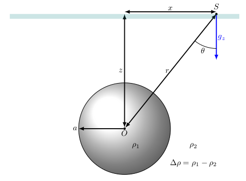
The gravity anomaly due to the buried sphere can be calculated using the following equations, \begin{align} g_z & = g_r \cos \theta\\ g_z & = \frac{GMz}{r^3}\\ g_z & = \frac{4 \pi G \Delta \rho a^3}{3} \frac{z}{(x^2 + z^2)^{3/2}} \end{align} where,
- $G$ is the gravitational constant
- $\Delta \rho$ is the density contrast between the sphere and surrounding material kg m$^{-3}$
- $a$ is the sphere radius (m)
- $x$ is horizontal distance from the sphere center (m)
- $z$ is depth from the surface to the sphere center (m)
Model assumptions
This model assumes that:
- The depth of the center of the sphere is greater than the sphere radius.
- The sphere is uniform and the density contrast between the sphere and the surrounding rock (or other material) is constant.
Model calculations
perl script
This perl script calculates the gravity anomaly due to a buried sphere using some example values for the parameters shown in the above model. The script requires an additional library, Math::SigFigs, to output the calculated gravity value with an appropriate number of significant figures. This library can be installed with the perl installer, cpan.
#!/usr/bin/perl
# USAGE: perl buried_sphere.pl > buried_sphere.dat

use warnings;
use strict;
use Math::SigFigs;

# Define some example constants
my $sphere_radius = 4000; #m
my $sphere_depth = 5000; #m (sphere_depth > sphere_radius)
my $sphere_density_contrast = 500; #kg/m3

for (my $i=0; $i<=10; $i++) {
  my $offset = $i * 1000; #horizontal distance (m)
  my $gravity = gsphere($sphere_radius, $sphere_depth, $offset, $sphere_density_contrast);

  print "$offset ";
  print FormatSigFigs($gravity,3), "\n";
}

###################################################################
#subroutine to calculate the gravity anomaly due to a buried sphere

# inputs:
#  sphere radius (m),
#  sphere depth (m),
#  calculation point:
#      horizontal distance from center of sphere to measurement(m)
#  density constrast (kg/m3)
# output:
#   gravity anomaly (mGal)
###################################################################
sub gsphere ($$$$) {

  my $pi = 3.14159265358979;
  my $a = shift;           # radius of the sphere (m)
  my $z = shift;           # depth of the center of the sphere (m)
  my $x = shift;           # horizontal distance of the
                           # location of the gravity observation (m)

  my $del_density = shift; # density cotrast (kg/m3)
  my $big_G = 6.67e-11;    #gravitational const.
  my $to_mgal = 1e5;       #convert SI to mGal

  my $V = (4/3)* $pi * $a ** 3;
  my $grav = $to_mgal * $big_G * $del_density * $V * $z * (($z*$z + $x*$x) ** (-3/2));

  return $grav;
};
p5.js script
This p5.js script creates the animation shown above. The script calculates the gravity anomaly due to the buried sphere shown in the figure above and plots the gravity values along the surface line.
// USAGE:
// Add these two script lines to the html header section:
// <script src="http://cdnjs.cloudflare.com/ajax/libs/p5.js/0.5.6/p5.js"><script>
// Here, the script source is with the html page
// <script src="canvas_gravity_sphere.js"><script>
//
// Add this div line to the html body section:
// <div id="sketch-holder" style="position: relative;"><div>

// The following is the script source code
var x = 100;
var y = 100;
var radius =  50; //in screen units, 1 km = 100 screen units
var x_zero = 50;
var x_scale = 100; //1 km = 100 screen units
var depth_zero = 200; //where the depth axis starts in screen units
var depth_scale = 100; //keep vert exaggeration 1:1
var mgal_zero = 170;  //less than depth_zero
var mgal_scale = 20;
var density_contrast = 500.0;

let myFont;
function preload() {
	// Font file is DejaVuSans.ttf,
	// copied to web page directory
  myFont = loadFont('DejaVuSans.ttf');
}

function setup() {
  var canvas = createCanvas(600,550);

  // Move the canvas so it's inside our div tag:
  // div id="sketch-holder"
  canvas.parent('sketch-holder');

  fill(0)
   .strokeWeight(.25);
  textFont(myFont, 16);
}

function draw() {
  background('#006747');

 var gravity;
 var x1km, y1km, r;
 var del_grav;
 var offset;
 var x1,  z1, m;
  // lerp() calculates a number between two numbers at a specific increment.
  // The amt parameter is the amount to interpolate between the two values
  // where 0.0 equal to the first point, 0.1 is very near the first point, 0.5
  // is half-way in between, etc.

  // Here we are moving 5% of the way to the mouse location each frame
  x = lerp(x,mouseX,0.05);
  y = lerp(y,mouseY,0.05);

  if (x < x_zero+radius) {x = x_zero + radius;}
  if (x > width - radius) {x = width - radius;}
  if (y < depth_zero+radius) {y = depth_zero + radius;}

  ellipse(x, y, 2*radius, 2*radius);

  // calculate and draw gravity
  // count in screen units
  for (offset = x_zero; offset < width; offset += 10) {

     x1 = (x) - offset;
     z1 = (y);

     x1km = x1 / x_scale * 1000.0;
     y1km = (z1 - depth_zero) / depth_scale * 1000.0;
     r = radius / x_scale * 1000.0;

     gravity =gsphere(r, x1km, y1km, density_contrast);

    // convert gravity to integer
    del_grav = gravity * mgal_scale;
     m = mgal_zero - del_grav;
    // plot point
    ellipse(offset, m, 6);
  }

  //draw axes and labels
  drawAxes(x_zero, x_scale, depth_zero, depth_scale, mgal_zero, mgal_scale);
}

function drawAxes(x_zero, x_scale, depth_zero, depth_scale, mgal_zero, mgal_scale) {
 fill('#CFC493');
 textAlign(RIGHT);
 for (var i = 0; i < 8; i++) {
  var d = i * depth_scale + depth_zero;
  line(x_zero, d, x_zero - 10, d);
  text(i, x_zero - 12, d + 5);
 }

 //draw and label mgal axis
 textAlign(RIGHT);
 for (var i = 0; i < 8 ; i++) {
  var d= mgal_zero - 2 * i * mgal_scale;
  line(x_zero, d, x_zero - 10, d);
  text(i * 2, x_zero - 12, d + 5);
 }

  //draw label the horizontal axis
  textAlign(CENTER);
  for (var i = 0; i < 12; i++) {
    var x = i * x_scale + x_zero;
    line(x, depth_zero - 35, x, depth_zero - 25);
    line(x, depth_zero-5, x, depth_zero + 5);
    var x_value =  i;
    text(x_value, x, depth_zero - 10);
  }

  // rotate(3.14159/2.0);
   textAlign(CENTER);
   text("z (km)", 100, 350);
   text("x (km)", 500, depth_zero+25);
   text("g (mgal)", 100, 100);
   stroke(255);
   fill(255);
   //depth arrow
   line(75, 360, 75, 400);
   triangle(70, 400, 80, 400, 75, 425);
    //horiontal arrow
   line(520, depth_zero+20, 555, depth_zero+20);
   triangle(555, depth_zero + 15, 555, depth_zero + 25, 580, depth_zero + 20);
    //mgal arrow
   line(75,80, 75, 40);
   triangle(70,40,80,40,75,15);
}

/*************************
calculate the gravity
  anomaly due to a sphere

  g-sphere = 4/3 rho G pi a^3 (1/(x^2+^2) (z)/(sqrt(x^2+z^2))
  distance units in meters
  returns mgal

  a = radius of sphere;
  x1 is horizontal offset
  z1 is depth;
***************************/
function gsphere(a, x2, z2, del_density){

  var g;
  var pi;
  var grav;

  //define consts.
  g = 6.67e-11;
  pi = 3.14159265358979;
  grav = 4.0/3.0 * pi * g * del_density * 1.0e5 * a * a * a * 1/(x2 * x2 + z2 * z2) * z2/(sqrt(x2 * x2 + z2 * z2));

  return grav; //return gravity in mgal
}
Drawing with LaTeX and TikZ
The following LaTeX and TikZ code draws the figure of the model geometry presented at the top of the page.
\documentclass{article}
\usepackage{tikz}
\usetikzlibrary{calc,fadings,decorations.pathreplacing}
\usetikzlibrary{shadings}
\usepackage{verbatim}
\usepackage{verbatim}
\usepackage[active,tightpage]{preview}
\PreviewEnvironment{tikzpicture}
\setlength\PreviewBorder{5pt}%
\begin{comment}

:Title: Buried sphere gravity anomaly
Illustrate the variables used and geometry
to calculate the gravity anomaly due to a buried sphere

Thanks to Tomasz M. Trzeciak and Latex-Community.org for
providing the key examples to get started on this code
\end{comment}

%% helper macros

\newcommand\pgfmathsinandcos[3]{%
  \pgfmathsetmacro#1{sin(#3)}%
  \pgfmathsetmacro#2{cos(#3)}%
}
\newcommand\LongitudePlane[3][current plane]{%
  \pgfmathsinandcos\sinEl\cosEl{#2} % elevation
  \pgfmathsinandcos\sint\cost{#3} % azimuth
  \tikzset{#1/.estyle={cm={\cost,\sint*\sinEl,0,\cosEl,(0,0)}}}
}
\newcommand\LatitudePlane[3][current plane]{%
  \pgfmathsinandcos\sinEl\cosEl{#2} % elevation
  \pgfmathsinandcos\sint\cost{#3} % latitude
  \pgfmathsetmacro\yshift{\cosEl*\sint}
  \tikzset{#1/.estyle={cm={\cost,0,0,\cost*\sinEl,(0,\yshift)}}} %
}
\newcommand\DrawLongitudeCircle[2][1]{
  \LongitudePlane{\angEl}{#2}
  \tikzset{current plane/.prefix style={scale=#1}}
   % angle of "visibility"
  \pgfmathsetmacro\angVis{atan(sin(#2)*cos(\angEl)/sin(\angEl))} %
  \draw[current plane] (\angVis:1) arc (\angVis:\angVis+180:1);
  \draw[current plane,dashed] (\angVis-180:1) arc (\angVis-180:\angVis:1);
}
\newcommand\DrawLatitudeCircle[2][1]{
  \LatitudePlane{\angEl}{#2}
  \tikzset{current plane/.prefix style={scale=#1}}
  \pgfmathsetmacro\sinVis{sin(#2)/cos(#2)*sin(\angEl)/cos(\angEl)}
  % angle of "visibility"
  \pgfmathsetmacro\angVis{asin(min(1,max(\sinVis,-1)))}
  \draw[current plane] (\angVis:1) arc (\angVis:-\angVis-180:1);
  \draw[current plane,dashed] (180-\angVis:1) arc (180-\angVis:\angVis:1);
}

%% document-wide tikz options and styles

\tikzset{%
  >=latex, % option for nice arrows
  inner sep=0pt,%
  outer sep=2pt,%
  mark coordinate/.style={inner sep=0pt,outer sep=0pt,minimum size=3pt,
    fill=black,circle}%
}

\begin{document}
\begin{tikzpicture} % "THE GLOBE" showcase

\def\Rone{2.0} % sphere1 radius
\def\Rtwo{5} % sphere1 radius
\def\angEl{35} % elevation angle
\filldraw[ball color=white] (0,0) circle (\Rone);

\def\angEl{25} % elevation angle
\def\angPhi{-40} % longitude of point P
\def\angPhitwo{-180} % longitude of point Q

\def\angBeta{30} % latitude of point  P and Q

\LongitudePlane[pzplane]{\angEl}{\angPhi}
\LongitudePlane[pqplane]{\angEl}{\angPhitwo}

\path[pqplane] (\Rone,0) coordinate (Q);
\coordinate [mark coordinate](O) at (0,0);
\coordinate [mark coordinate](S) at (4,5);
\node[below] at (O) {$O$};
\node[above=4 pt] at (S) {$S$};

\draw[->, very thick] (O) -- (Q) node[left]{$a$};
\draw[<->, very thick] (O) -- node[left]{$z$} (0,5) ;
\draw[<->, very thick] (O) -- node[left]{$r$} (4,5) ;
\draw[<->, very thick] (0,5.1) -- node[above]{$x$} (4,5.1) ;
\draw[teal, line width = 6, opacity = 0.2] (-5,4.9) --  (5,4.9) ;
\draw[blue, very thick, ->] (S) -- node[right]{$g_z$} (4,3);
\draw [black] (4,3.5) arc [radius=1.5, start angle=-90, end angle= -129];

 \node at (3.4,3.4) {$\theta$};
 \node at (3,-0.75) {$\rho_2$};
 \node at (0.5,-0.75) {$\rho_1$};
 \node at (3,-1.5) {$\Delta \rho = \rho_1 - \rho_2$};
\end{tikzpicture}
\end{document}
Some References
- Telford, W.M., Geldart, L.P. and Sheriff, R.E. (1990) Applied Geophysics, Cambridge University Press.
- MacMillan, W.D. (1958) The Theory of the Potential, Dover Books on Science and Engineering, New York.