Introduction to inversion
Learn about inversion using the magnetic anomaly of a sphere using a brute force approach
Contents
Introduction
Here we consider inversion for one parameter, depth of a buried sphere, using its magnetic anomaly. Since we are interested in one parameter, "brute force" works reasonably well. In brute force methods we simple search the entire problem space to find the best-fit value of a parameter.
In this example, the forward solution is the magnetic anomaly due to a buried sphere. A description of the forward model is available here.
Data Set
First we need data. In this example we actually use the forward model to calculate the expected magnetic anomaly of a sphere buried in the subsurface with known geometry and magnetic properties. To make the solution slightly more realistic, we add noise to the data set by randomly sampling a normal distribution with zero mean and 25 nT standard deviation. This is added to the forward solution to produce an artificial magnetic anomaly that is noisy, but relatively easy to model.
Here is the example dataset: mag_sphere.dat
Here is the example dataset: mag_anomaly_sphere_data_struct.c
and here is a code to plot these data using gnuplot: mag_sphere.gnuThis data set is a magnetic anomaly that looks like:
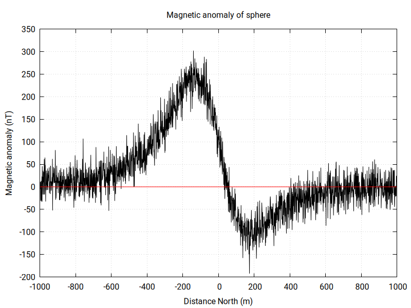
The black curve on the graph shows the "data", for the noisy magnetic anomaly on a North-South transect across a buried sphere located at point (0,0). The red line shows data values for the calculated anomaly determined by inversion, which is currently zero since the inversion is not done yet.
Forward Solution
Consider a C function that calculates the forward solution - given x,y, position, depth, radius, and the vector of magnetization, return the calculated magnetic anomaly. The function is:
C code
    /*
A function to calculate the magnetic anomaly due to a sphere

C. Connor
Feb, 2025

*/

double magnetized_sphere_anomaly(double x, double y, Sphere sphere) {
    double minc = sphere.minc * M_PI / 180.0; // Inclination down in rad
    double mdec = sphere.mdec * M_PI / 180.0; // Declination east in rad

    double ml = cos(minc) * cos(mdec);
    double mm = cos(minc) * sin(mdec);
    double mn = sin(minc);

    double dpm = (4.0 / 3.0) * M_PI * pow(sphere.a, 3) * sphere.mi;

    double mx = sphere.mi * ml;
    double my = sphere.mi * mm;
    double mz = sphere.mi * mn;

    double einc = sphere.einc * M_PI / 180.0; // Inclination down in rad
    double edec = sphere.edec * M_PI / 180.0; // Declination east in rad

    double el = cos(einc) * cos(edec);
    double em = cos(einc) * sin(edec);
    double en = sin(einc);

    double prop = 400 * M_PI;

    double z = - sphere.z;

    x = x - sphere.easting;
    y = y - sphere.northing;

    double r2 = x * x + y * y + z * z;
    double r = sqrt(r2);
    double r5 = pow(r, 5);

    double dotprod = x * mx + y * my + z * mz;

    double bx = prop * dpm * (3 * dotprod * x - r2 * mx) / r5;
    double by = prop * dpm * (3 * dotprod * y - r2 * my) / r5;
    double bz = prop * dpm * (3 * dotprod * z - r2 * mz) / r5;

    return el * bx + em * by + en * bz;
}
Given a x,y location at the surface, where a magnetic value is calculated, the function returns the magnetic anomaly due to a sphere. Note the function takes a data structure called Sphere as one of its arguments, that has all of the information (parameters) used to calculate the anomaly.
Sphere Struct code
The Sphere data struct looks like:
/* Define the Sphere data structure
  for magnetic anomaly calculation
  */
typedef struct {
    double northing;  // northing coordinate of the sphere center (m)
    double easting;    // easting coordinate of the sphere center (m)
    double z; // depth to sphere center (m)
    double a; // radius of the sphere (m)
    double minc; //inclination of the vector of magnetization of the sphere (degrees)
    double mdec; //inclination of the vector of magnetization of the sphere (degrees)
    double mi; //intensity of the vector of magnetization of the sphere (amp/m)
    double einc; //inclination of the Earth's magnetic field (degrees)
    double edec; //declination of the Earth's magnetic field (degrees)
} Sphere;
The inversion method
The inversion uses a brute force method. In this case we are inverting for the depth of the center of the sphere. We have no other information, so we invert from 0.1 m depth to 1000 m depth, assuming this range is sufficient: that the true depth lies between these two values. We calculate the forward model 100 times at different depths within this range and print out the root-mean-square-error (RMSE) value for each calculation. The lowest RMSE is the "best-fit" estimate of the depth of the center of the sphere.
A flowchart that illustrates the "brute force" search looks like:
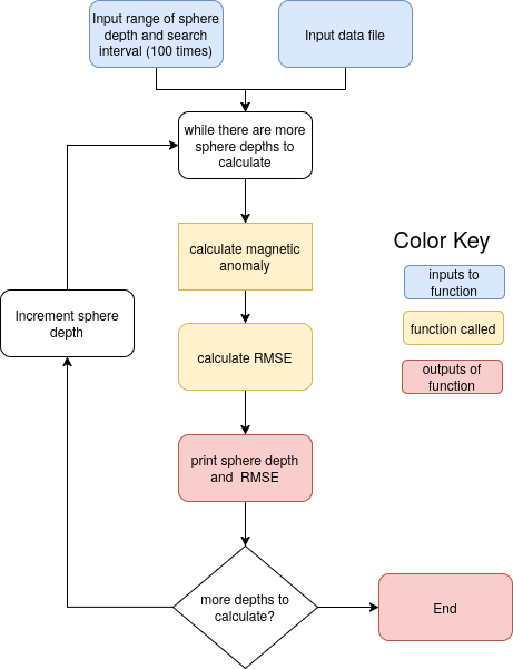
The blue-colored flowchart boxes are inputs to the brute force search function. The yellow-shaded boxes are functions that are called by the brute force search function (actually in this simple code RMSE can just be calculated inside the search fuction). The red-shaded box is the output of the search function - in this case just the depth and the RMSE are printed to the screen (which you can pipe to a datafile and plot).
The C method
The code that performs the inversion: mag_anomaly_brute_force_search.cTo compile the code type:
gcc -o brute mag_anomaly_brute_force_search.c -lm
To run the code:
./brute
Be sure the data file mag_sphere.dat is in the same directory as the executable code. If all goes well, you should be able to plot the RMSE as a function of sphere depth. The plot should look like this one:
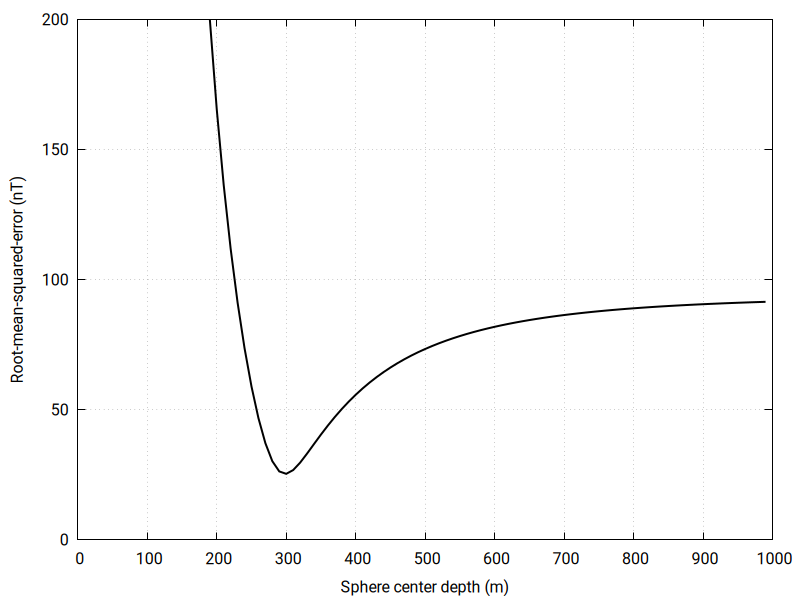
Note the minimum RMSE is close to the actual depth (the depth used to create the noisy magnetic anomaly with the forward solution). Recall that the standard deviation used to add noise to the "observed" magnetic anomaly was 25 nT. The RMSE for the best-fit solution is also about 25 nT, indicating the only uncertainty in the model is due to the random error. Most inversions do not work out so well! But, if you use an analytical solution to generate an "observed" dataset and add noise, the best-fit RMSE should be roughly equal to the standard deviation of the noise you introduced. You can test inversion codes like this one to see if they converge on the noise you added.
Things to try
- Download the inversion code and dataset. Compile the code and run it. Pipe the the output to a data file and write a gnuplot script to illustrate the RMSE as a function of depth. What is the best-fit depth?
- Calculate a new forward solution using the best-fit RMSE and compare to the observed data
- Change the input dataset by increasing the variance of the noise. What happens to the RMSE value for the best-fit solution when the variance is increased?
- Modify the code so it inverts for a different parameter, like the magnitude of the vector of magnetization.