Deformation due to a buried point-like pressure source
Calcuate the expected deformation of a sub-surface radially symmetric and small-volume pressure source
Contents
Introduction
In 1958, Kiyoo Mogi published a paper in which he described remarkable deformation of Sakurajima volcano during and following its 1914 eruption. He documented subsidence following the eruption of tens of centimeters up to 17 km from the volcano's vent. The pattern of subsidence was radially symmetric about a point near the location of the volcanic vent, so Mogi realized the pattern of deformation provided insight about the change in pressure beneath the volcano during the eruption.
His paper is well-known today primarily because he went on to develop a model to describe the change in pressure within the Earth necessary to explain the observed radial pattern of deformation. The model is elegant in its simplifying assumptions and useful because deformation associated with a variety of processes, such as subsidence due to groundwater withdrawal, or inflation of volcanoes prior to some volcanic eruptions.
The calculation presented in the following is more fully explained in:
Connor, C., 2022. Computing for Numeracy: Kiyoo Mogi and the nature of volcanoes, Numeracy, 15(1)
Visualizing Mogi's model with p5
The following sketch illustrates Mogi's calculation for a sub-surface point-like pressure source. The sphere (large white circle in the illustration) represents the position of the point-like pressure source in the sub-surface. The mouse is used to change the position of the point-like source and the calculation is updated for the position. Adjust the excess pressure, $\Delta P$, using the slider bar. The deformation observed at the surface is shown in terms of vertical displacement ($w$, mm) (white small circles) and horizontal displacement ($u$, yellow small circles). Note that the sign of the horizontal displacement changes across the point-like source. To the left of the source the horizontal displacement is in the negative $x$-direction and to the right of the point-like source the displacement is in the positive $x$-direction. In other words, the displacement is radially symmetric with respect to the point-like source.
For this calculation, The radius of the point-like source is 0.5 km, the shear modulus, $G = 3 \times 10^5$ MPa, and Poisson's ratio is $\sigma = 0.25$.
Model calculations
The following image describes the geometry of the problem. The point-like source, centered on point $O$, has radius $a$ and is located at depth $d$, where $a << d$. The displacement is calculated at point $S$, located a radial distance $x$ from $O$. The point-like pressure source has excess pressure, $\Delta P$, which results in displacement at the Earth's surface (blue shaded line), which is described by the two vectors $w$ and $u$.
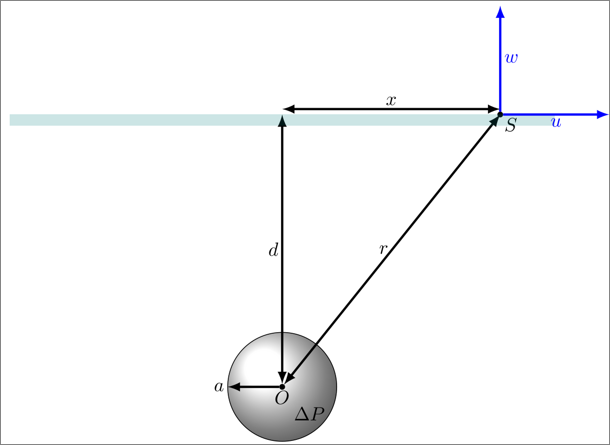
The surface displacements produced by change in hydrostatic pressure within a spherical cavity in two dimensions are given by: $$\begin{pmatrix}u\\w\end{pmatrix} = a^3\Delta P\frac{1-v}{G(x^2+d^2)^\frac{3}{2}} \begin{pmatrix}x\\d\end{pmatrix}$$ where:
Model assumptions
This model assumes that:
- The Earth's crust is an homogeneous, semi-infinite elastic half-space
- The origin of the pressure anomaly in the subsurface is a small spherical source.
p5.js script
This p5.js script creates the animation shown above. The script calculates the gravity anomaly due to the buried sphere shown in the figure above and plots the gravity values along the surface line.
// USAGE:
// Add these two script lines to the html header section:
// <script src="http://cdnjs.cloudflare.com/ajax/libs/p5.js/0.5.6/p5.js"><script>
// Here, the script source is with the html page
// <script src="surface_deformation.point.js"><script>
//
// Add this div line to the html body section:
// <div id="sketch-holder" style="position: relative;"><div>

// The following is the script source code

var x = 100;
var y = 100;
var radius =  20; //in screen units, 1 km = 40 screen units
var x_zero = 50;
var x_scale = 40; //1 km = 40 screen units
var initial_depth = 2; //initial depth in km
var depth_zero = 300; //where the depth axis starts in screen units
var depth_scale = 40; //keep vert exaggeration 1:1
var deformation_min = 270;  //less than depth_zero
var deformation_scale = 12;
var deformation_zero;
var del_pressure;
var slider;

function setup() {
  var canvas = createCanvas(600,650);

  // Move the canvas so it's inside our .
  canvas.parent('sketch-holder');
//  canvas.noStroke();
  slider = createSlider(10, 40, 2);
  slider.parent('slider');
  slider.position(width-190, 30);
  slider.style('width','180px','background','white');
  fill(0)
   .strokeWeight(.25);
  del_pressure = 10;
}

function draw() {
  background('#006747');

 var mogi = [];
 var x1km, y1km, r;
 var mogi_x, mogi_z;
 var offset;
 var x1,  z1, m, n;
 var del_pressure = slider.value();

  // lerp() calculates a number between two numbers at a specific increment.
  // The amt parameter is the amount to interpolate between the two values
  // where 0.0 equal to the first point, 0.1 is very near the first point, 0.5
  // is half-way in between, etc.

  // Here we are moving 5% of the way to the mouse location each frame
  //if (mouseX > 0 && mouseY > 0){
  x = lerp(x,mouseX,0.05);
  y = lerp(y,mouseY,0.05);//}

  if (x < x_zero+radius) {x = x_zero+radius;}
  if (x > width - radius) {x = width - radius;}
  if (y < depth_zero+2*radius) {y = depth_zero+2*radius;}
  if (y > height - radius) {y = height - radius;}
  ellipse(x, y, 2*radius, 2*radius);

  ////calculate and draw deformation
  for (offset=x_zero; offset< width; offset+=10){
     x1 = offset - (x);
     z1 = (y);
     x1km = x1/x_scale*1000.0;
     y1km = (z1 - depth_zero)/depth_scale*1000.0 +  initial_depth*1000.0;
     r = radius/x_scale*1000.0;

     mogi =gsphere(r, x1km, y1km, del_pressure);
     // convert deformation to integer
     mogi_x = mogi[0]*1000*deformation_scale;
     mogi_z = mogi[1]*1000*deformation_scale
     m = deformation_zero - mogi_z;
     n = deformation_zero - mogi_x;
     // plot point
     ellipse(offset, m, 6);
    fill('yellow');
     ellipse(offset, n, 6);
    fill(255)
  }
  //draw axes and labels
  drawAxes(x_zero, x_scale, depth_zero, depth_scale, deformation_min, deformation_scale, initial_depth);
}


function drawAxes(x_zero, x_scale, depth_zero, depth_scale, deformation_min, deformation_scale, d_i) {
 fill('#CFC493');
 textAlign(RIGHT);
 for (var i = 0; i< 9 ; i++) {
  var  d= i*depth_scale + depth_zero;
  line(x_zero,d,x_zero-10,d);
  text(i + d_i,x_zero-12,d+5);
 }

  //draw and label u,w axis
 textAlign(RIGHT);
 for (var i = 0; i< 11 ; i++) {
  var d= deformation_min - 2*i*deformation_scale;
  line(x_zero,d,x_zero-10,d);
  text(i*2 - 6,x_zero-12,d+5);
     if(i*2 - 6 == 0){deformation_zero = d;}
 }
  //draw label the horizontal axis
  textAlign(CENTER);
 for (var i = 0; i<14; i++) {
  var x=i*x_scale + x_zero;
  line(x,depth_zero-35,x,depth_zero-25);
  line(x,depth_zero-5,x,depth_zero+5);
  var x_value =  i;
   text(x_value,x,depth_zero-10);
 }
  // rotate(3.14159/2.0);
   textAlign(CENTER);
   text(slider.value(), width - 200, 40);
   text("Delta P (MPa)", width - 50, 20)

   text("z (km)", 100, 350);
   text("x (km)", 500, depth_zero+25);

   text("w (mm)", 100, 100);
  fill('yellow')
   text("u (mm)", 100, 120);

   stroke(255);
   fill(255);
   //depth arrow
   line(75, 360, 75, 400);
   triangle(70,400,80,400,75,425);
    //horiontal arrow
   line(520, depth_zero+20, 555, depth_zero+20);
   triangle(555,depth_zero+15,555,depth_zero+25,580,depth_zero+20);
    //mgal arrow
   line(75,80, 75, 40);
   triangle(70,40,80,40,75,15);
}


function gsphere(a, x2, z2, del_pressure){

  var G;
  var u;
  var w;

/*calculate the surface
deformation due to a point pressure source

u=  3.0/4.0 * del_pressure * r * a**3 / (G * (r**2 + d**2)**(3/2));
w=  3.0/4.0 * del_pressure * d * a**3 / (G * (r**2 + d**2)**(3/2));
distance units in meters
returns meters

a = radius of sphere;
x1 is horizontal offset
z1 is depth;
*/
//define consts.
G=30000; //shear modulus in MPa
u=  3.0/4.0 * del_pressure * x2 * pow(a, 3) / (G * pow(pow(x2,2) + pow(z2, 2), 3/2));
w=  3.0/4.0 * del_pressure * z2 * pow(a, 3) / (G * pow(pow(x2,2) + pow(z2, 2), 3/2));

return [u,w]; //return x, z displacement in meters
}
python script
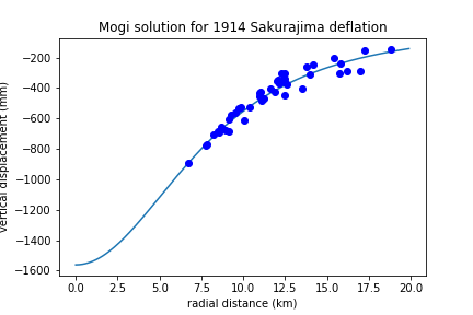
The following python code calculates the vertical displacement using the Mogi solution as a function. The calculated displacement is compared with the data collected on deflation of Sakurajima volcano following the 1914 eruption. The survey data were collected using precise line levelling. The displacements are found by calculating the differences in elevations at permanent survey markers between surveys in 1893 and 1914, following the eruption. The data indicate there was dramatic deflation of the volcano edifice following the 1914 eruption, likely due to depressurization of a magma reservoir. The survey data were collected by F. Omori and were reported in Mogi (1958).
The script includes python functions for vertical and horizontal displacements. It is necessary to have python modules installed to run the script. The modules required are:
- matplotlib
- numpy
The python script can be cut and paste into a jupyter notebook, or run using any python v3+ environment.
import numpy as np
import matplotlib.pyplot as plt

def mogi_vertical(x,a,d,g,delta_p,sigma):
    # Calculate the vertical displacement (m)
    # at the surface due to a subsurface
    # pressure source using Mogi's solution
    # x is horizontal distance (m), radial from source
    # a is source radius (m) must be << d
    # d is depth (m)
    # g is shear modulus (MPa), typically 3e5 or less
    # delta_p is the excess pressure of the source (MPa)
    # sigma is Poisson's ratio (typically 0.25)
    w = (1-sigma)*a**3*d*delta_p/(g*(x**2+d**2)**1.5)
    return w  # m displacement

def mogi_horizontal(x,a,d,g,delta_p,sigma):
    # calculate the horizontal displacement (m) at the
    # the surface due to a subsurface pressure
    # source using Mogi's solution.
    # x is horizontal distance (m), radial from source
    # a is source radius (m) must be << d
    # d is depth (m)
    # g is shear modulus (MPa), typically 3e5 or less
    # delta_p is the excess pressure of the source (MPa)
    # sigma is Poisson's ratio (typically 0.25)
    u = (1-sigma)*a**3*x*delta_p/(g*(x**2+d**2)**1.5)
    return u # m displacement

a = 2500.0 #source radius (m)
d = 10000.0 #source depth (m)
sigma = 0.25 #Poisson ratio
delta_p = -400.0 #excess pressure (MPa)
g = 30000.0 #rigidity of elastic half-space (MPa)

# Sakurajima displacements following 1914 eruption
# The data are taken from Mogi (1958)
# The data were collected by line levellin by
# F. Omori and colleagues
# displacement is the difference between
# measured elevations in 1893 and 1914.
sakura = [(17.0,-291),
(16.2,-291),
(15.75,-302),
(13.5,-407),
(12.45,-446),
(10.4,-527),
(8.7,-658),
(7.85,-770),
(6.7,-894),
(7.75,-776),
(8.25,-703),
(9.15,-608),
(9.85,-526),
(9.7,-536),
(9.55,-560),
(9.3,-577),
(8.5,-684),
(8.55,-690),
(8.95,-681),
(9.15,-685),
(10.05,-616),
(11.1,-481),
(11.9,-427),
(12.15,-369),
(12.1,-348),
(12.5,-301),
(12.3,-306),
(10.95,-433),
(11.05,-426),
(11.0,-453),
(12.0,-356),
(12.4,-344),
(12.5,-363),
(11.6,-401),
(11.2,-468),
(12.6,-379),
(13.95,-314),
(15.8,-242),
(12.15,-369),
(12.5,-338),
(13.75,-260),
(14.15,-244),
(15.4,-206),
(17.25,-155),
(18.8,-143)]

# calculate vertical displacement for this
# range of radial distances (m)
x1 = np.arange(0,20000,100)

# plot vertical displacement calculated with
# Mogi solution in mm vs. km
plt.plot(x1/1000, mogi_vertical(x1,a,d,g,delta_p,sigma)*1000)

# Compare the Mogi solution to observations
# for Salurajima following deflation after
# the 1914 eruption
radial, vert_displace = zip(*sakura)
plt.plot(radial, vert_displace, "bo")
plt.xlabel("radial distance (km)")
plt.ylabel("vertical displacement (mm)")
plt.title("Mogi solution for 1914 Sakurajima deflation")
plt.savefig("sakurajima.png")
plt.show()
python script output
The python script outputs this figure, showing the calculated vertical displacement (blue line) as a function of distance from the center of deflation. The displacement data collected by Omori are shown as solid blue circles. Changing the model parameters in the python script will change the fit between the Mogi model and Omori's observations.
Drawing with LaTeX and TikZ
The following LaTeX and TikZ code draws the figure of the model geometry presented at the top of the page.
\documentclass{article}
\usepackage{tikz}
\usetikzlibrary{calc,fadings,decorations.pathreplacing}
\usetikzlibrary{shadings}

\usepackage{verbatim}
\usepackage{verbatim}
\usepackage[active,tightpage]{preview}
\PreviewEnvironment{tikzpicture}
\setlength\PreviewBorder{5pt}%
\begin{comment}

:Title: Mogi source
Illustrate the variables used and geometry
to calculate the displacement due to a small buried sphere

Thanks to Tomasz M. Trzeciak and Latex-Community.org for
providing the key examples to get started on this code

\end{comment}

%% helper macros

\newcommand\pgfmathsinandcos[3]{%
  \pgfmathsetmacro#1{sin(#3)}%
  \pgfmathsetmacro#2{cos(#3)}%
}
\newcommand\LongitudePlane[3][current plane]{%
  \pgfmathsinandcos\sinEl\cosEl{#2} % elevation
  \pgfmathsinandcos\sint\cost{#3} % azimuth
  \tikzset{#1/.estyle={cm={\cost,\sint*\sinEl,0,\cosEl,(0,0)}}}
}
\newcommand\LatitudePlane[3][current plane]{%
  \pgfmathsinandcos\sinEl\cosEl{#2} % elevation
  \pgfmathsinandcos\sint\cost{#3} % latitude
  \pgfmathsetmacro\yshift{\cosEl*\sint}
  \tikzset{#1/.estyle={cm={\cost,0,0,\cost*\sinEl,(0,\yshift)}}} %
}
\newcommand\DrawLongitudeCircle[2][1]{
  \LongitudePlane{\angEl}{#2}
  \tikzset{current plane/.prefix style={scale=#1}}
   % angle of "visibility"
  \pgfmathsetmacro\angVis{atan(sin(#2)*cos(\angEl)/sin(\angEl))} %
  \draw[current plane] (\angVis:1) arc (\angVis:\angVis+180:1);
  \draw[current plane,dashed] (\angVis-180:1) arc (\angVis-180:\angVis:1);
}
\newcommand\DrawLatitudeCircle[2][1]{
  \LatitudePlane{\angEl}{#2}
  \tikzset{current plane/.prefix style={scale=#1}}
  \pgfmathsetmacro\sinVis{sin(#2)/cos(#2)*sin(\angEl)/cos(\angEl)}
  % angle of "visibility"
  \pgfmathsetmacro\angVis{asin(min(1,max(\sinVis,-1)))}
  \draw[current plane] (\angVis:1) arc (\angVis:-\angVis-180:1);
  \draw[current plane,dashed] (180-\angVis:1) arc (180-\angVis:\angVis:1);
}

%% document-wide tikz options and styles

\tikzset{%
  >=latex, % option for nice arrows
  inner sep=0pt,%
  outer sep=2pt,%
  mark coordinate/.style={inner sep=0pt,outer sep=0pt,minimum size=3pt,
    fill=black,circle}%
}

\begin{document}

\begin{tikzpicture} % "THE GLOBE" showcase

\def\Rone{1.0} % sphere1 radius
\def\Rtwo{5} % sphere1 radius
\def\angEl{35} % elevation angle
\filldraw[ball color=white] (0,0) circle (\Rone);

\def\angEl{25} % elevation angle
\def\angPhi{-40} % longitude of point P
\def\angPhitwo{-180} % longitude of point Q

\def\angBeta{30} % latitude of point  P and Q

\LongitudePlane[pzplane]{\angEl}{\angPhi}
\LongitudePlane[pqplane]{\angEl}{\angPhitwo}


\path[pqplane] (\Rone,0) coordinate (Q);

\coordinate [mark coordinate](O) at (0,0);
\coordinate [mark coordinate](S) at (4,5);
\node[below] at (O) {$O$};
\node[below right] at (S) {$S$};


\draw[->, very thick] (O) -- (Q) node[left]{$a$};
\draw[<->, very thick] (O) -- node[left]{$d$} (0,5) ;
\draw[<->, very thick] (O) -- node[left]{$r$} (4,5) ;
\draw[<->, very thick] (0,5.1) -- node[above]{$x$} (4,5.1) ;
\draw[teal, line width = 6, opacity = 0.2] (-5,4.9) --  (5,4.9) ;

\draw[blue, very thick, ->] (S) -- node[right]{$w$} (4,7);
\draw[blue, very thick, ->] (S) -- node[below]{$u$} (6,5);


 \node at (0.5,-0.5) {$\Delta P$};

\end{tikzpicture}

\end{document}
Some References
- Mogi, K. 1958. Relations between the eruptions of various volcanoes and the deformations of the ground surfaces around them. Earthq Res Inst, 36, pp.99-134.
- Dzurisin, D., 2006. Volcano deformation: new geodetic monitoring techniques. Springer Science and Business Media.