The Gravity Anomaly at Aso Caldera
Results of modeling gravity at Aso Caldera using inversion with the gbox model
Introduction
Grav-parallel is a C code written in parallel (with MPI) designed to model the gravity anomaly due to a body that can be represented by prisms. The code assumes that the prisms have a uniform top depth and uniform density contrast. The code models the depth to the bottom of each prism.
The gbox forward model is used. The inversion is done using the Ameoba algorthim, also called the Nedler-Meade simplex method.
[Top]
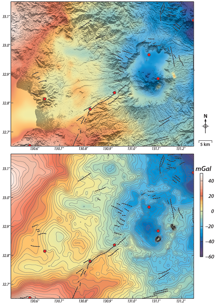
Regional complete Bouguer gravity anomaly for the area around Aso caldera, superimposed on a shaded-relief digital elevation model (top) and contoured (bottom). The caldera is characterized by a prominent large-amplitude gravity low centered west of Nakedake, an active vent within the caldera (red dot). Other vents in the volcano database of Japan are shown as red dots including Omine and Akai volcanoes, west of the caldera boundary. Faults, from the Quaternary fault database of Japan are shown as dashed lines, including the Futagawa fault zone segment, which connects Akai and Omine volcanoes and trends into Aso caldera. Figure courtesy of L. Connor.
Aso caldera

[Top]
inversion model inputs
inversion model outputs
observed input gravity contoured
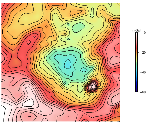
modeled gravity contoured
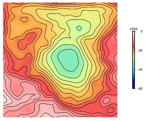
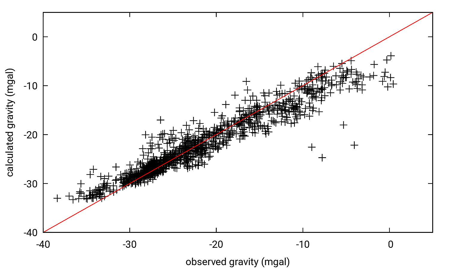
equiline plot of observed gravity vs. calculated gravity values
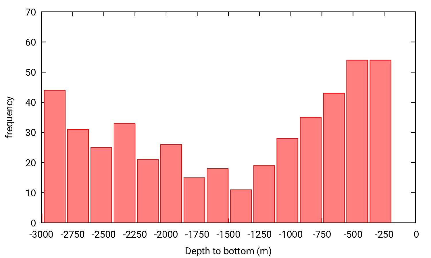
histogram of the depths of all prisms
3D model and corresponding colored contours of prism bottoms
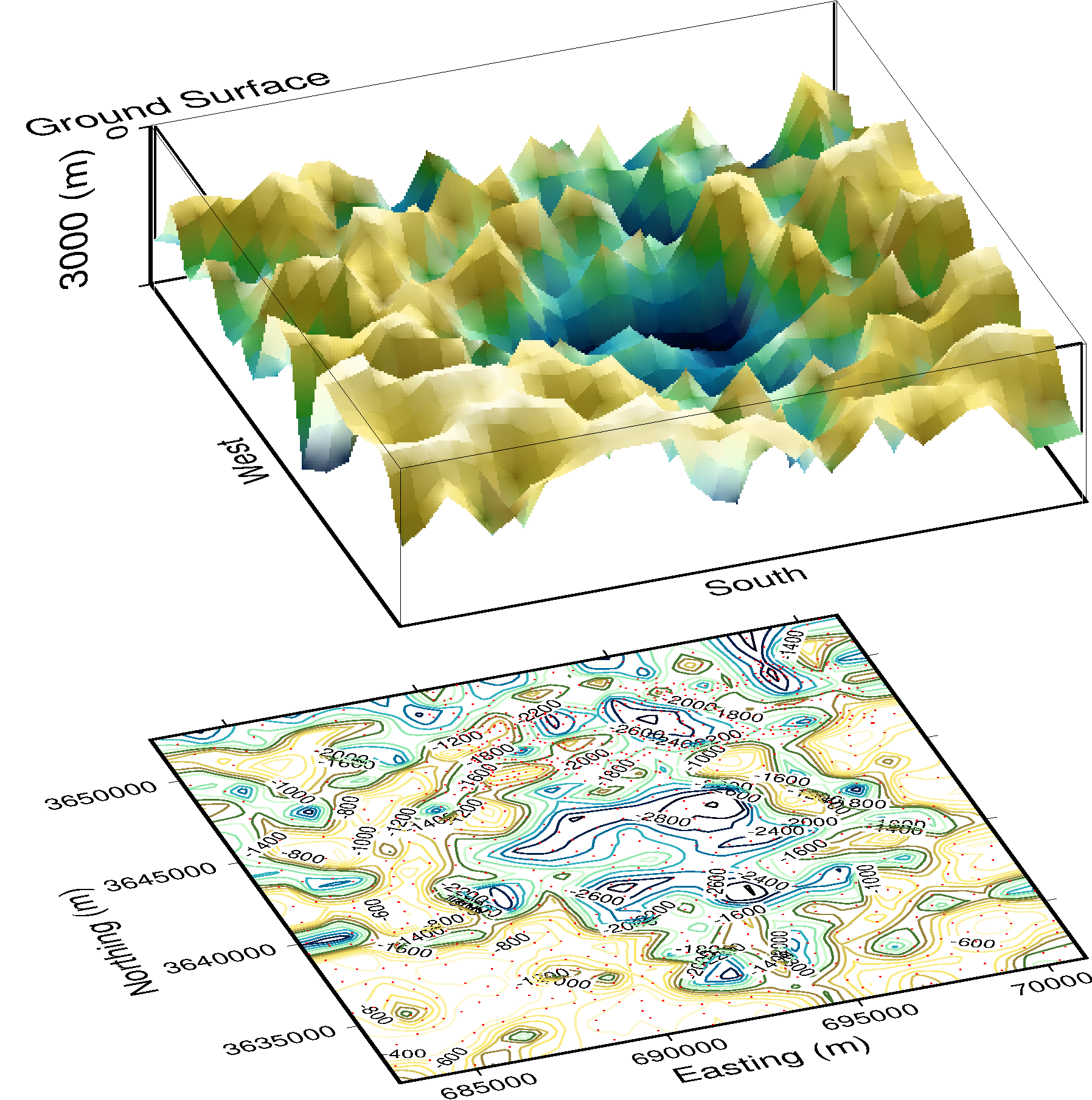
Preliminary Aso Results
TOLERANCE 1.0e-3
SEED 13
# The following three values are used in building
# the anomaly of prisms.
# The first value is the minimum, the second is the maximum.
MIN_NORTHING 3630500
MAX_NORTHING 3653500
MIN_EASTING 682000
MAX_EASTING 701500
SPACING 1000
MIN_ROC_DENSITY -800.0
MAX_ROC_DENSITY -300.0
MIN_DEPTH_TO_BOTTOM 100.0
MAX_DEPTH_TO_BOTTOM 3000.0
MIN_DEPTH_TO_TOP 100.0
MAX_DEPTH_TO_TOP 800.0
Fri Apr 10 14:11:47 2020

Best RMSE = 2.5
	682000.000000 to 701500.000000 (Easting)
	3630500.000000 to 3653500.000000 (Northing)
	Spacing = 1000.0 (meters)

Number of Parameters = 380
Number of Vertices = 381
Tolerance = 0.001000
Parameter Ranges:
	Rock Density: -800 -300
	Depth-to-top: 100.00  800.00
	Depth-to-bottom: 100.00  3000.00

Modeled Anomaly:
	Depth to Tallest Prism: 2989.99 (meters)
	Top Depth: 229.01(meters)
		Rock Density: -470.92


[Top]
Reference: https://gscommunitycodes.usf.edu/geoscicommunitycodes/public/geophysics/Gravity/gravparallel.php
Some References
- Bott, M.H.P., 1960. The use of rapid digital computing methods for direct gravity interpretation of sedimentary basins. Geophysical Journal International, 3(1), pp.63-67.
- Telford, W.M., Geldart, L.P. and Sheriff, R.E. (1990) Applied Geophysics, Cambridge University Press.
- Blakely, R. J., 1996, Potential Theory in Gravity and Magnetic Applications, Cambridge University Press
- Plouff, D., 1976, Gravity and magnetic fields of polygonal prisms and application to magnetic terrain corrections. Geophysics 41: 727-741.
Citation
Connor, C. B. (2020) C code for calculating the gravity anomaly due to a vertical-sided prism.Reference: https://gscommunitycodes.usf.edu/geoscicommunitycodes/public/geophysics/Gravity/gravparallel.php