Gravity anomaly due to a horizontal cylinder

Contents

• Mathematical model
• Model assumptions
• Calculating and plotting an anomaly with gnuplot
• Drawing the model geometry using LaTeX and TikZ
• References and citation

Introduction

The gravity anomaly due to a horizontal cylinder may be used to approximate the gravity anomaly due to a buried tunnel, lava tube, or karst conduit. The trick to developing this model is to realize that the Gaussian surface enclosing the cylinder can be expressed in terms of surface area per unit length along the cylinder, as can the mass per unit length. This works if the cylinder is infinite, in other words, the ends are ignored.

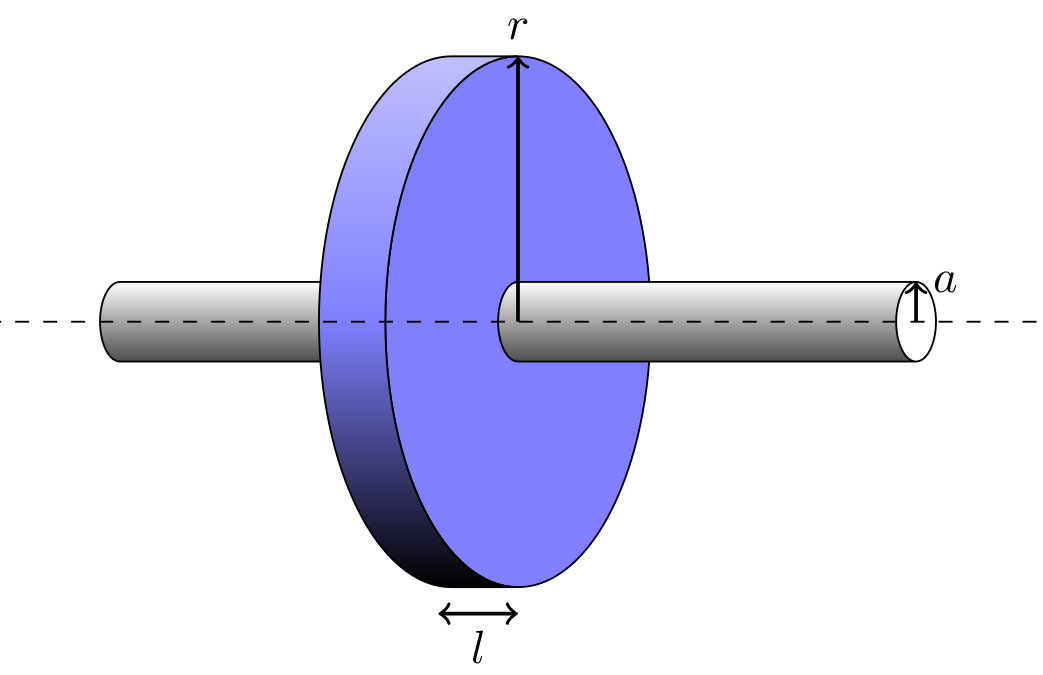
The blue disk in this figure represents the hypothetical Gaussian surface, of radius $r$. Because the vector of gravity due to the cylinder is oriented toward the axis of the cylinder in the plane of the disk, the surface integral is the circumference of the blue disk times its unit length, $l$.

Mathematical model

Estimate the gravity anomaly, $g$, due to an infinite horizontal cylinder using Gauss's law, \begin{align} \oint_S \vec g \cdot \vec n dA & = -4 \pi GM\\ M_l & = \pi a^2 \Delta \rho\\ -2 \pi r l g & = -4 \pi G M_l l\\ g & = \frac{2GM_l}{r}\\ g & = \frac{2G \pi a^2 \Delta \rho}{r} \end{align} where:

• $M_l$ is the mass per unit length of the cylinder and
• $\Delta \rho$ is the density contrast between the cylinder and the surrounding rock.
• $a$ is the radius of the cylinder
• $G$ is the gravitational constant
• $r$ is the distance from the center of the cylinder to the point where $g$ is determined

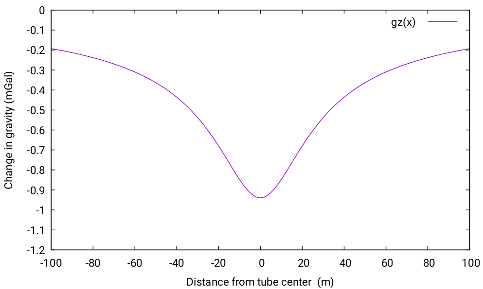
Calculate and plot the anomaly using gnuplot

The following gnuplot script plots the gravity anomaly due to a horizontal cylinder. Experiment with different constant values for:

• the density contrast, $\rho$
• the cylinder radius, $a$
• the depth to the center of the cylinder axis, $z$

# USAGE: gnuplot hort.gnu
# (to be run on the command line)

set termoption dash
Grv = 6.67e-11 #gravitational constant
rho = -2400 #density contrast (kg m-3)
a = 14 #radius (m)
z= 21 #depth to center (m)
gz(x) = 2*Grv*pi*a**2*rho/(x**2 + z**2)**0.5 * 1e5

# Axes label
set xlabel 'Distance from tube center  (m)'
set ylabel 'Change in gravity (mGal)'

# Axes ranges
set xrange [-100:100]
set yrange [-1.2:0]

# Axes tics
set xtics 20
set ytics 0.1
set tics scale 0.75
set key Left

plot gz(x)
set term pdf enhanced dashed
set output "hort_cylinder_graph.pdf"

Drawing with LaTeX and TikZ

The following LaTeX and TikZ code draws the figure of the model geometry presented at the top of the page.

\documentclass{article}
\usepackage{tikz}
\usetikzlibrary{calc,fadings,decorations.pathreplacing}
\usepackage{verbatim}
\usepackage{verbatim}
\usepackage[active,tightpage]{preview}
\PreviewEnvironment{tikzpicture}
\setlength\PreviewBorder{5pt}%

\begin{document}
\begin{tikzpicture}

\draw[top color=white,bottom color=black!70] (0,3mm) arc (90:270:1.5mm and 3mm)--++(-3cm,0) arc (-90:-270:1.5mm and 3mm)-- cycle;
\draw[fill=blue!50](0,0) circle (1 and 2);
\draw[top color=blue!25,bottom color=black,middle color=blue!50] (-0.5,2) arc (90:270:1 and 2) -- ++(0.5,0) arc (-90:-270:1 and 2) -- cycle;
\draw[top color=white,bottom color=black!70] (0,3mm) arc (90:270:1.5mm and 3mm)--++(3cm,0) arc (-90:-270:1.5mm and 3mm)-- cycle;
\draw (3cm,3mm) arc (90:-90:1.5mm and 3mm);
\draw [dashed] (-4 cm, 0 mm) -- ( 4cm, 0 mm);
\draw[thick, ->] (3 cm, 0 mm) -- ( 3cm, 3 mm)  node[right] {$a$};
\draw[thick, ->] (0 cm, 0 mm) -- ( 0cm, 2)  node[above] {$r$};
\draw[thick, <->] (-6 mm, -2.2) --  node[below] {$l$} ( 0cm, -2.2);
\end{tikzpicture}

\end{document}